Analysis of Noise In Communication Systems

ANALYSIS OF NOISE IN COMMUNICATION SYSTEMS:

·        Thermal Noise (Johnson noise)

It has been discussed that the thermal noise in a resistance R has a mean square value given by

Where k = Boltzmann‘s constant = 1.38 x 10-23 Joules per K

T = absolute temperature

B = bandwidth noise measured in (Hz)

R = resistance (ohms)

This is found to hold for large bandwidth (>1013 Hz) and large range in temperature. This thermal noise may be represented by an equivalent circuit as shown below.

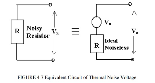
i.e. equivalent to the ideal noise free resistor (with same resistance R) in series with a voltage source with voltage Vn.

Since

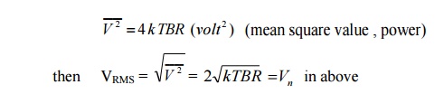
i.e. Vn is the RMS noise voltage.

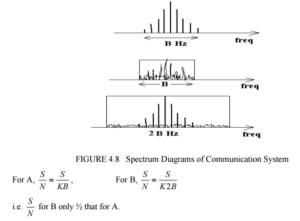
The above equation indicates that the noise power is proportional to bandwidth. For a given resistance R, at a fixed temperature T (Kelvin)

For a given system, with (4 k TR)     constant, then if we double the bandwidth from B Hz to 2B Hz, the noise power will double (i.e increased by 3 dB). If the bandwidth were increased by a factor of 10, the noise power is increased by a factor of 10.For this reason it is important that the system bandwidth is only just ‗wide‘ enough to allow the signal to pass to limit the noise bandwidth to a minimum.

Ø I.e. Signal Spectrum Signal Power = S

A) System BW = B Hz

N= Constant B (watts) = KB

B) System BW

N= Constant 2B (watts) = K2B

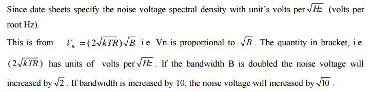
 Noise Voltage Spectral Density 

 Resistance in Series

 Series Assume that R1 at temperature T1 and R2 at temperature T2, then

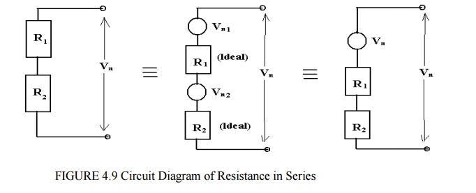
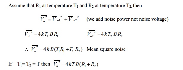
i.e. The resistor in series at same temperature behave as a single resistor  (R1 + R2)

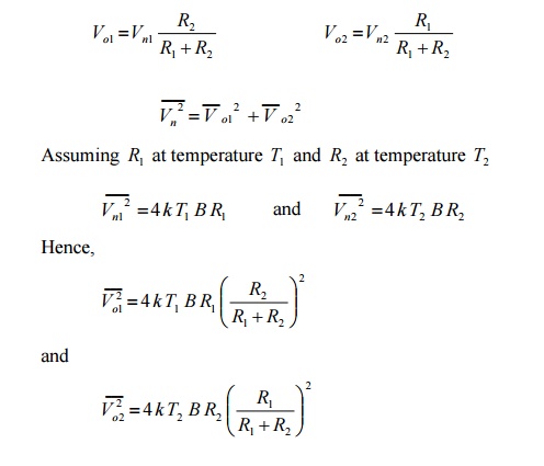
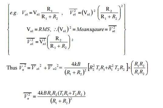
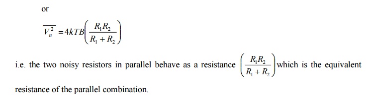
ü   Resistance in Parallel

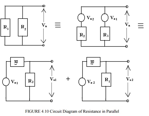
Since an ideal voltage source has zero impedance, we can find noise as an output Vo1, due to Vn1 , an output voltage V02 due to Vn2.

ü   MATCHED COMMUNICATION SYSTEMS:

In communication systems we are usually concerned with the noise (i.e. S/N) at the receiver end of the system.

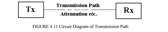
The transmission path may be for example:-

a)  A transmission line (e.g. coax cable).

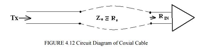
Zo is the characteristics impedance of the transmission line, i.e. the source resistance Rs. This is connected to the receiver with an input impedance RIN .

b) A radio path (e.g. satellite, TV, radio – using aerial)

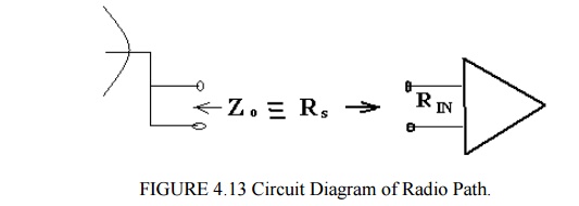
Again Zo=Rs the source resistance, connected to the receiver with input resistance Rin. Typically Zo is 600 ohm for audio/ telephone systems

Or Zo is 50 ohm (for radio/TV systems) 75 ohm (radio frequency systems).

An equivalent circuit, when the line is connected to the receiver is shown below. (Note we omit the noise due to Rin – this is considered in the analysis of the receiver section).

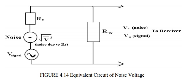
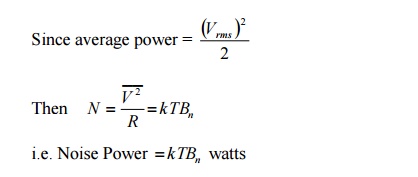
For a matched system, N represents the average noise power transferred from the source to the load. This may be written as

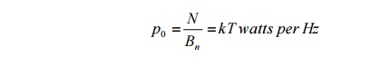
where  p0  is the noise power spectral density (watts per Hz)

Bn is the noise equivalent bandwidth (Hz) k is the Boltzmann‘s constant

T is the absolute temperature K.

Note: that p0  is independent of frequency, i.e. white noise.

These equations indicate the need to keep the system bandwidth to a minimum, i.e. to that required to pass only the band of wanted signals, in order to minimize noise power, N.

For example, a resistance at a temperature of 290 K (17 deg C), p0 = kT is 4 x 10-21 watts per Hz. For a noise bandwidth Bn = 1 KHz, N is 4 x 10-18 watts (-174 dBW).If the system bandwidth is increased to 2 KHz, N will decrease by a factor of 2 (i.e. 8 x 10-18 watts or -171 dBW) which will degrade the (S/N) by 3 dB.Care must also be exercised when noise or (S/N ) measurements are made, for example with a power meter or spectrum analyser, to be clear which bandwidth the noise is measured in, i.e. system or test equipment. For example, assume a system bandwidth is 1 MHz and the measurement instrument bandwidth is 250 KHz.

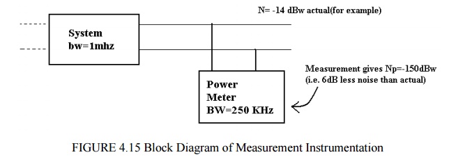
In the above example, the noise measured is band limited by the test equipment rather than the system, making the system appears less noisy than it actually is. Clearly if the relative bandwidths are known (they should be) the measured noise power may be corrected to give the actual noise power in the system bandwidth.

If the system bandwidth was 250 KHz and the test equipment was 1 MHz then the measured result now would be – 150 dBW (i.e. the same as the actual noise) because the noise power monitored by the test equipment has already been band limited to 250 KHz.

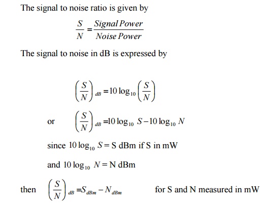
ü   SIGNAL – TO – NOISE : 

ü  NOISE FACTOR – NOISE FIGURE:

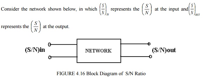
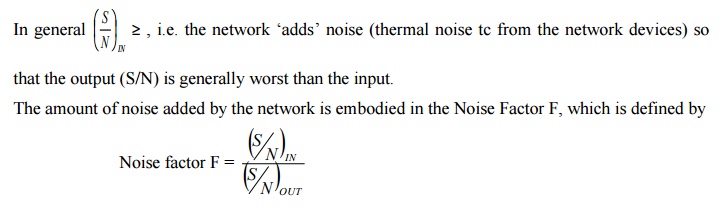
F equals to 1 for noiseless network and in general F > 1. The noise figure in the noise factor quoted in dB

i.e. Noise Figure F dB = 10 log10 F   F ≥ 0 dB

The noise figure / factor is the measure of how much a network degrades the (S/N)IN, the lower the value of F, the better the network.

The network may be active elements, e.g. amplifiers, active mixers etc, i.e. elements with gain > 1 or passive elements, e.g. passive mixers, feeders cables, attenuators i.e. elements with gain <1.

ü   NOISE FIGURE – NOISE FACTOR FOR ACTIVE ELEMENTS :

For active elements with power gain G>1, we have

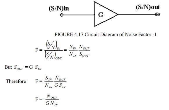
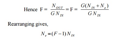
If the NOUT was due only to G times N IN  the F would be 1 i.e. the active element would be noise free. Since in general F v> 1 , then NOUT  is increased by noise due to the active element i.e.

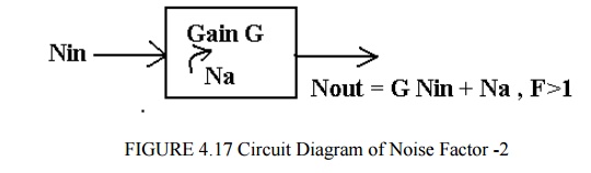
Na represents ‘added‘ noise measured at the output. This added noise may be referred to the input as extra noise, i.e. as equivalent diagram is

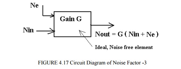
Ne is extra noise due to active elements referred to the input; the element is thus effectively noiseless.

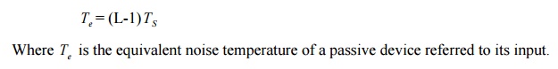
ü NOISE TEMPERATURE:

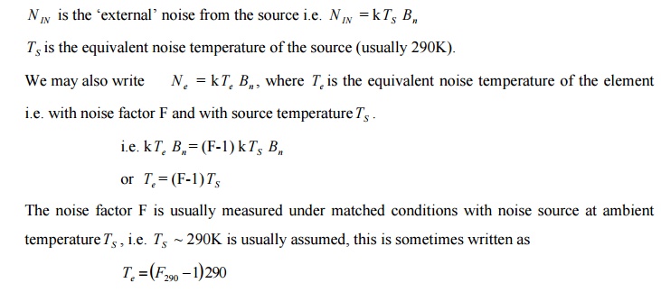
This allows us to calculate the equivalent noise temperature of an element with noise factor F, measured at 290 K.

For example, if we have an amplifier with noise figure FdB = 6 dB (Noise factor F=4) and equivalent Noise temperature Te = 865 K.

·        Comments:-

a)     We have introduced the idea of referring the noise to the input of an element, this noise is not actually present at the input, it is done for convenience in the analysis.

b)    The noise power and equivalent noise temperature are related, N=kTB, the temperature T is not necessarily the physical temperature, it is equivalent to the temperature of a resistance R (the system impedance) which gives the same noise power N when measured in the same bandwidth Bn.

c)     Noise figure (or noise factor F) and equivalent noise temperature Te are related and both indicate how much noise an element is producing.

Since,  Te = (F-1) TS

Then for F=1, Te = 0, i.e. ideal noise free active element.

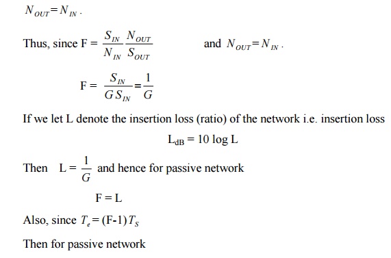
ü   NOISE FIGURE – NOISE FACTOR FOR PASSIVE ELEMENTS :

The theoretical argument for passive networks (e.g. feeders, passive mixers, attenuators) that is networks with a gain < 1 is fairly abstract, and in essence shows that the noise at the input, N IN is attenuated by network, but the added noise Na contributes to the noise at the output such that

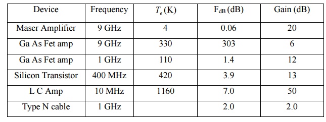
 REVIEW OF NOISE FACTOR – NOISE FIGURE –TEMPERATURE:

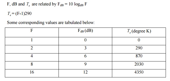
Typical values of noise temperature, noise figure and gain for various amplifiers and attenuators are given below:

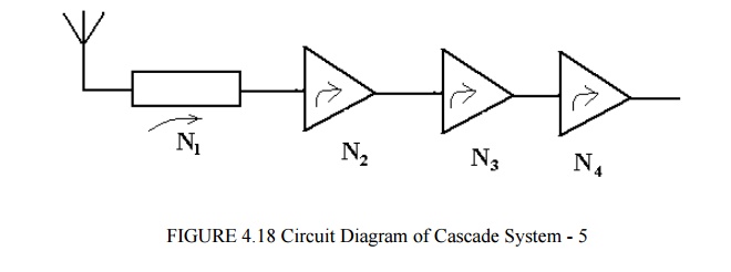
ü   CASCADED NETWORK:

A receiver systems usually consists of a number of passive or active elements connected in series, each element is defined separately in terms of the gain (greater than 1 or less than 1 as the case may be), noise figure or noise temperature and bandwidth (usually the 3 dB bandwidth). These elements are assumed to be matched.

A typical receiver block diagram is shown below, with example

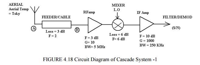
In order to determine the (S/N) at the input, the overall receiver noise figure or noise temperature must be determined. In order to do this all the noise must be referred to the same point in the receiver, for example to A, the feeder input or B, the input to the first amplifier.

The equations so far discussed refer the noise to the input of that specific element i.e.

Te  or N e is the noise referred to the input.

To refer the noise to the output we must multiply the input noise by the gain G. For example, for a lossy feeder, loss L, we had

N e = (L-1) N IN , noise referred to input Or Te = (L-1) TS - referred to the input.

Noise referred to output is gain x noise referred to input, hence

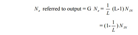
Similarly, the equivalent noise temperature referred to the output is

These points will be clarified later; first the system noise figure will be considered.

ü   SYSTEM NOISE FIGURE:

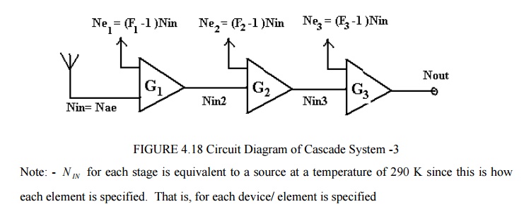
Assume that a system comprises the elements shown below, each element defined and specified separately.

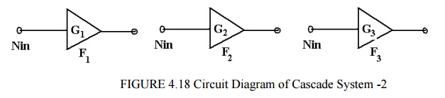
The gains may be greater or less than 1, symbols F denote noise factor (not noise figure, i.e. not in dB). Assume that these are now cascaded and connected to an aerial at the input, with

N IN  = N ae  from the aerial.

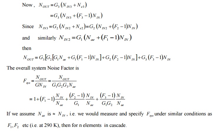
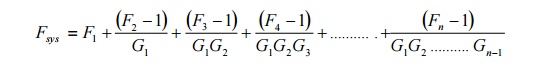
The equation is called FRIIS Formula.

This equation indicates that the system noise factor depends largely on the noise factor of the first stage if the gain of the first stage is reasonably large. This explains the desire for ―low noise front ends‖ or low noise most head preamplifiers for domestic TV reception. There is a danger however; if the gain of the first stage is too large, large and unwanted signals are applied to the mixer which may produce intermodulation distortion. Some receivers apply signals from the aerial directly to the mixer to avoid this problem. Generally a first stage amplifier is designed to have a good noise factor and some gain to give an acceptable overall noise figure.

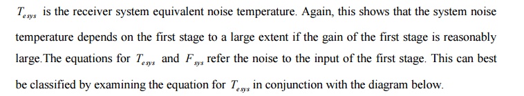
SYSTEM NOISE TEMPERATURE:

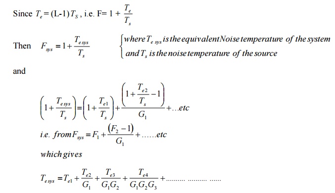
See examples and tutorials for further classifications.

ü   REVIEW AND APPLICATION:

It is important to realize that the previous sections present a technique to enable a receiver performance to be calculated. The essence of the approach is to refer all the noise contributed at various stages in the receiver to the input and thus contrive to make all the stages ideal, noise free. i.e. in practice or reality : -

The noise gets worse as we proceed from the aerial to the output. The technique outlined.

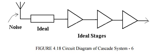
All noise referred to input and all stages assumed noise free.

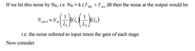
To complete the analysis consider the system below

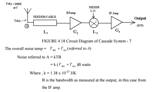
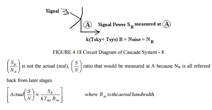
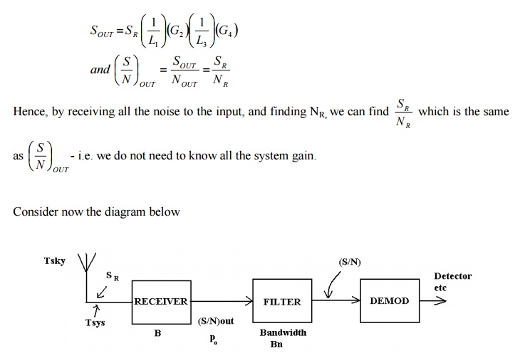
A filter in same form often follows the receiver and we often need to know po , the noise power spectral density.

i.e. recall that N= po B = kTB. po = kT

We may find  po  from

po  = k( T sky  + T sys  )

ü   ALGEBRAIC REPRESENTATION OF NOISE:

·        General

In order for the effects of noise to be considered in systems, for example the analysis of probability of error as a function of Signal to noise for an FSK modulated data systems, or the performance of analogue FM system in the presence of noise, it is necessary to develop a model which will allow noise to be considered algebraically.

Noise may be quantified in terms of noise power spectral density po watts per Hz such that the average noise power in a noise bandwidth Bn Hz is

N=  po Bn watts

Thus the actual noise power in a system depends on the system bandwidth and since we are often

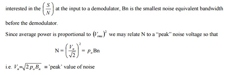
In practice noise is a random signal with (in theory) a Gaussian distribution and hence peak values up to ± ¥ or as otherwise limited by the system dynamic range are possible. Hence this ―peak‖ value for noise is a fictitious value which will give rise to the same average noise as the actual noise.

·        PHASOR REPRESENTATION OF SIGNAL AND NOISE:

shown below:

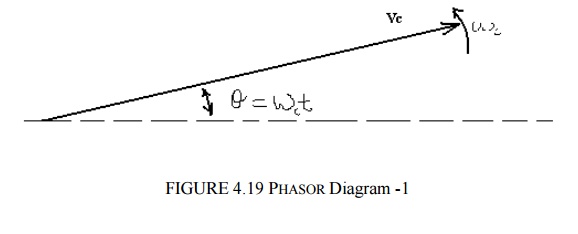
The phasor represents a signal with peak value Vc, rotating with angular frequencies Wc rads per sec and with an angle q = wc t to some reference axis at time t=0.

If we now consider a carrier with a noise voltage with ―peak‖ value superimposed we may represents this as:

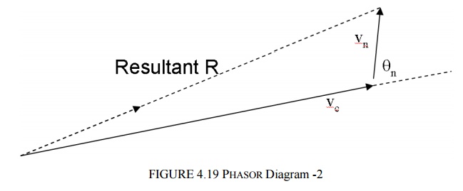
In this case Vn is the peak value of the noise and is the phase of the noise relative to the carrier. Both Vn and q n are random variables, the above phasor diagram represents a snapshot at some instant in time.

The resultant or received signal R, is the sum of carrier plus noise. If we consider several snapshots overlaid as shown below we can see the effects of noise accompanying the signal and how this affects the received signal R.

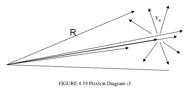
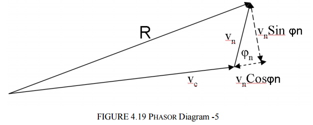
Thus the received signal has amplitude and frequency changes (which in practice occur randomly) due to noise.We may draw, for a single instant, the phasor with noise resolved into 2 components, which are:

a)  x(t) in phase with the carriers

x(t) =Vn Cosfn

b)  y(t) in quadrature with the carrier

y(t) = Vn Sinfn

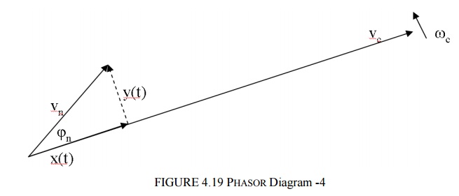
The reason why this is done is that x(t) represents amplitude changes in Vc (amplitude changes affect the performance of AM systems) and y(t) represents phase (i.e. frequency) changes (phase / frequency changes affect the performance of FM/PM systems)

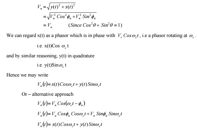
We note that the resultant from x(t) and y(t) i.e.

We can regard x(t) as a phasor which is in phase with Vc Cos wc t , i.e a phasor rotating at wc . i.e. x(t)Cos wc t

and by similar reasoning, y(t) in quadrature i.e. y(t)Sin wc t

Hence we may write

Vn (t )= x(t) Coswc t + y(t) Sinwc t

Or – alternative approach

Vn (t )= Vn Cos(wc t -fn )

Vn (t )= Vn Cosfn Coswc t +Vn  Sinfn  Sinwc t

Vn (t )= x(t) Coswc t + y(t) Sinwc t

This equation is algebraic representation of noise and since

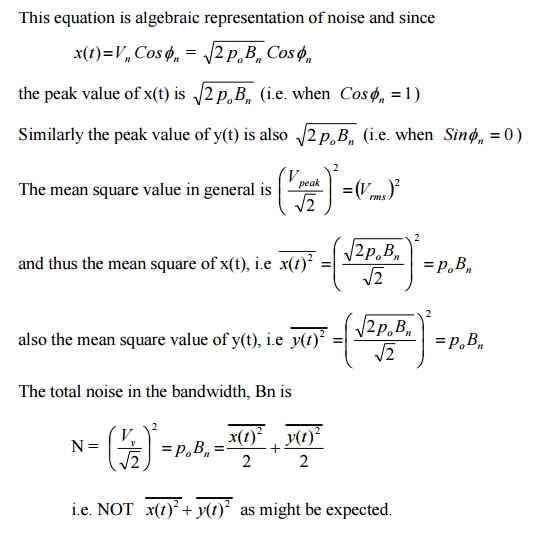
The reason for this is due to the Cosfn and Sinfn relationship in the representation e.g. when say ―x(t)‖ contributes   po Bn , the ―y(t)‖ contribution is zero, i.e. sum is always equal to  po Bn .

The algebraic representation of noise discussed above is quite adequate for the analysis of many systems, particularly the performance of ASK, FSK and PSK modulated systems.

When considering AM and FM systems, assuming a large (S/N) ratio, i.e Vc>> Vn, the following may be used.

Considering the general phasor representation below:-

For AM systems, the signal is of the form (Vc + m(t))Coswc t where m(t) is the message or modulating signal and the resultant for (S/N) >> 1 is

AM received = (Vc + m(t))Coswc t + x(t) Coswc t

Since AM is sensitive to amplitude changes, changes in the Resultant length are predominantly due to x(t).

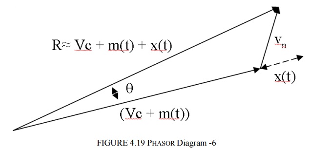
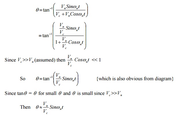
For FM systems the signal is of the form Vc Cos(wc ± Dw)t . Noise will produce both amplitude changes (i.e. in Vc) and frequency variations – the amplitude variations are removed by a limiter in the FM receiver. Hence,

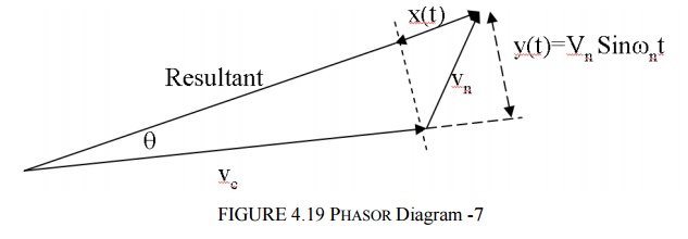
The angle q represents frequency / phase variations in the received signal due to noise. From the diagram.

The above discussion for AM and FM serve to show bow the ‘model‘ may be used to describe the effects of noise.Applications of this model to ASK, FSK and PSK demodulation, and AM and FM demodulation are discussed elsewhere.

ü   ADDITIVE WHITE GAUSSIAN NOISE:

Noise in Communication Systems is often assumed to be Additive White Gaussian Noise (AWGN).

·        Additive

Noise is usually additive in that it adds to the information bearing signal. A model of the received signal with additive noise is shown below.

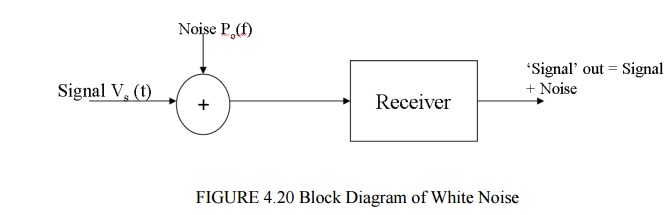
The signal (information bearing) is at its weakest (most vulnerable) at the receiver input. Noise at the other points (e.g. Receiver) can also be referred to the input.The noise is uncorrelated with the signal, i.e. independent of the signal and we may state, for average powers

Output Power = Signal Power + Noise Power

= (S+N)

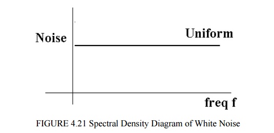
·        White

As we have stated noise is assumed to have a uniform noise power spectral density, given that the noise is not band limited by some filter bandwidth.

We have denoted noise power spectral density by po ( f ). White noise = po (f )= Constant

Also Noise power =  po Bn

·        GAUSSIAN

We generally assume that noise voltage amplitudes have a Gaussian or Normal distribution.