Method of Least Squares

METHOD OF LEAST SQUARES

In most of the cases, the data points do not fall on a straight line (not highly correlated), thus leading to a possibility of depicting the relationship between the two variables using several different lines. Selection of each line may lead to a situation where the line will be closer to some points and farther from other points. We cannot decide which line can provide best fit to the data.

Method of least squares can be used to determine the line of best fit in such cases. It determines the line of best fit for given observed data by minimizing the sum of the squares of the vertical deviations from each data point to the line.

1. Method of Least Squares

To obtain the estimates of the coefficients ‘a’ and ‘b’, the least squares method minimizes the sum of squares of residuals. The residual for the i^th data point e_i is defined as the difference between the observed value of the response variable, y_i, and the estimate of the response variable, ŷ_i, and is identified as the error associated with the data. i.e., e_i = y_i–ŷ_i , i =1 ,2, ..., n.

The method of least squares helps us to find the values of unknowns ‘a’ and ‘b’ in such a way that the following two conditions are satisfied:

Sum of the residuals is zero. That is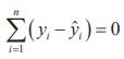 

Sum of the squares of the residuals E ( a , b ) =  is the least

2. Fitting of Simple Linear Regression Equation

The method of least squares can be applied to determine the estimates of ‘a’ and ‘b’ in the simple linear regression equation using the given data (x₁,y₁), (x₂,y₂), ..., (x_n,y_n) by minimizing

Here, yˆi = a + bx _i is the expected (estimated) value of the response variable for given x_i.

It is obvious that if the expected value (y^{^} _i) is close to the observed value (y_i), the residual will be small. Since the magnitude of the residual is determined by the values of ‘a’ and ‘b’, estimates of these coefficients are obtained by minimizing the sum of the squared residuals, E(a,b).

Differentiation of E(a,b) with respect to ‘a’ and ‘b’ and equating them to zero constitute a set of two equations as described below:

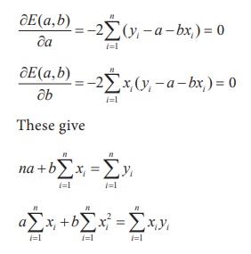
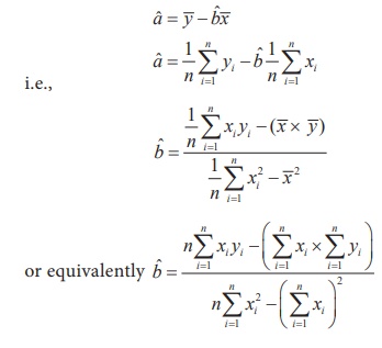
These equations are popularly known as normal equations. Solving these equations for ‘a’ and ‘b’ yield the estimates ˆa and ˆb.

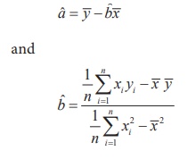
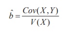
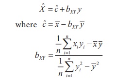
It may be seen that in the estimate of ‘ b’, the numerator and denominator are respectively the sample covariance between X and Y, and the sample variance of X. Hence, the estimate of ‘b’ may be expressed as

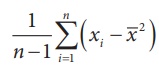
Further, it may be noted that for notational convenience the denominator of b^ˆ above is mentioned as variance of _nX. But, the definition of sample variance remains valid as defined in Chapter I, that is,

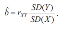
From Chapter 4, the above estimate can be expressed using, r_XY , Pearson’s coefficient of the simple correlation between X and Y, as

Important Considerations in the Use of Regression Equation:

1. Regression equation exhibits only the relationship between the respective two variables. Cause and effect study shall not be carried out using regression analysis.

2. The regression equation is fitted to the given values of the independent variable. Hence, the fitted equation can be used for prediction purpose corresponding to the values of the regressor within its range. Interpolation of values of the response variable may be done corresponding to the values of the regressor from its range only. The results obtained from extrapolation work could not be interpreted.

Example 5.1

Construct the simple linear regression equation of Y on X if 

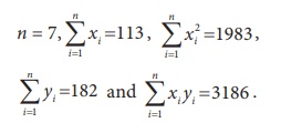
Solution:

The simple linear regression equation of Y on X to be fitted for given data is of the form

 ˆY = a + bx               ……..(1)

The values of ‘a’ and ‘b’ have to be estimated from the sample data solving the following normal equations.

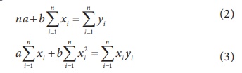
Substituting the given sample information in (2) and (3), the above equations can be expressed as

7 a + 113 b = 182 (4)

113 a + 1983 b = 3186 (5)

(4) × 113 ⇒ 791 a + 12769 b = 20566

(5) × 7 ⇒ 791 a + 13881 b = 22302

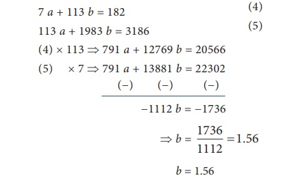
Substituting this in (4) it follows that,

7 a + 113 × 1.56 = 182

7 a + 176.28 = 182

7 a = 182 – 176.28

= 5.72

Hence, a = 0.82

Example 5.2

Number of man-hours and the corresponding productivity (in units) are furnished below. Fit a simple linear regression equation ˆY = a + bx applying the method of least squares.

Solution:

The simple linear regression equation to be fitted for the given data is

ˆY^ˆ = a + bx

Here, the estimates of a and b can be calculated using their least squares estimates

From the given data, the following calculations are made with n=9

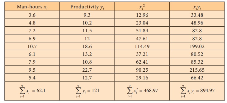
Substituting the column totals in the respective places in the of the estimates aˆ and b^ˆ , their values can be calculated as follows:

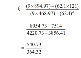
Thus, b^ˆ = 1.48 .

Now aˆ can be calculated using b^ˆ as

aˆ = 121/9 – (1.48× 62.1/9)

= 13.40 – 10.21

Hence, aˆ = 3.19

Therefore, the required simple linear regression equation fitted to the given data is

ˆY^ˆ = 3.19 +1.48x

It should be noted that the value of Y can be estimated using the above fitted equation for the values of x in its range i.e., 3.6 to 10.7.

In the estimated simple linear regression equation of Y on X

ˆY^ˆ = aˆ + ˆbx

we can substitute the estimate aˆ =  − b^ˆ . Then, the regression equation will become as

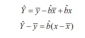
It shows that the simple linear regression equation of Y on X has the slope b^ˆ and the corresponding straight line passes through the point of averages (  , ). The above representation of straight line is popularly known in the field of Coordinate Geometry as ‘Slope-Point form’. The above form can be applied in fitting the regression equation for given regression coefficient b^ˆ and the averages  and  .

As mentioned in Section 5.3, there may be two simple linear regression equations for each X and Y. Since the regression coefficients of these regression equations are different, it is essential to distinguish the coefficients with different symbols. The regression coefficient of the simple linear regression equation of Y on X may be denoted as b_YX and the regression coefficient of the simple linear regression equation of X on Y may be denoted as b_XY.

Using the same argument for fitting the regression equation of Y on X, we have the simple linear regression equation of X on Y with best fit as

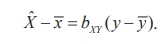
The slope-point form of this equation is

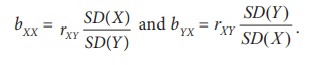
Also, the relationship between the Karl Pearson’s coefficient of correlation and the regression coefficient are