Fiber dispersion measurements

Fiber dispersion measurements

Dispersion measurements give an indication of the distortion to optical signals as they propagate down optical fibers. The delay distortion which, for example, leads to the broadening of transmitted light pulses limits the information-carrying capacity of the fiber. The measurement of dispersion allows the bandwidth of the fiber to be determined. Therefore, besides attenuation, dispersion is the most important transmission characteristic of an optical fiber. As discussed in Section 3.8, there are three major mechanisms which produce dispersion in optical fibers (material dispersion, waveguide dispersion and intermodal dispersion). The importance of these different mechanisms to the total fiber dispersion is dictated by the fiber type. For instance, in multimode fibers (especially step index), intermodal dispersion tends to be the dominant mechanism, whereas in single-mode fibers intermodal dispersion is nonexistent as only a single mode is allowed to propagate. In the single-mode case the dominant dispersion mechanism is chromatic (i.e. intramodal dispersion). The dominance of intermodal dispersion in multimode fibers makes it essential that dispersion measurements on these fibers are performed only when the equilibrium mode distribution has been established within the fiber, otherwise inconsistent results will be obtained. Therefore devices such as mode scramblers or filters must be utilized in order to simulate the steady state mode distribution.

Dispersion effects may be characterized by taking measurements of the impulse response of the fiber in the time domain, or by measuring the baseband frequency response in the frequency domain. If it is assumed that the fiber response is linear with regard to power, a mathematical description in the time domain for the optical output power Po(t) from the fiber may be obtained by convoluting the power impulse response h(t) with the optical input power Pi(t) as:

where the asterisk * denotes convolution. The convolution of h(t) with Pi(t) shown in Eq. (4.6) may be evaluated using the convolution integral where:

In the frequency domain the power transfer function H(w) is the Fourier transform of h(t) and therefore by taking the Fourier transforms of all the functions in Eq. (4.6) we obtain:

1. Time domain measurement

The most common method for time domain measurement of pulse dispersion in multimode optical fibers is illustrated in Figure 4.9. Short optical pulses (100 to 400 ps) are launched into the fiber from a suitable source (e.g. A1GaAs injection laser) using fast driving electronics. The pulses travel down the length of fiber under test (around 1 km) and are broadened due to the various dispersion mechanisms. However, it is possible to take measurements of an isolated dispersion mechanism by, for example, using a laser with a narrow spectral width when testing a multimode fiber. In this case the chromatic dispersion is negligible and the measurement thus reflects only intermodal dispersion.

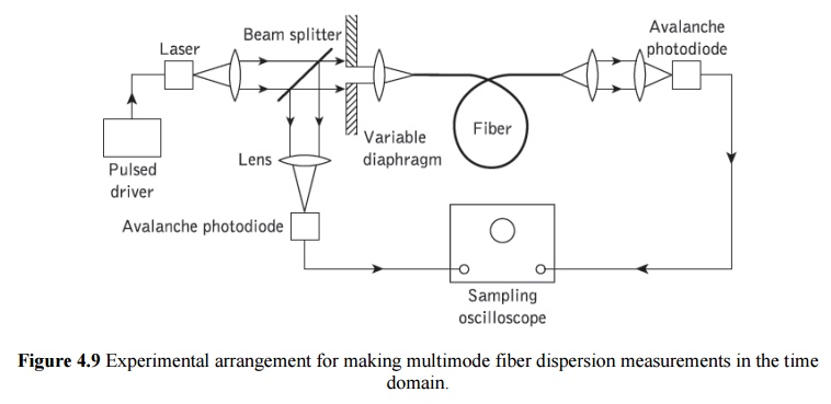
The pulses are received by a high-speed photodetector (i.e. avalanche photodiode) and are displayed on a fast sampling oscilloscope. A beam splitter is utilized for triggering the oscilloscope and for input pulse measurement. After the initial measurement of output pulse width, the long fiber length may be cut back to a short length and the measurement repeated in order to obtain the effective input pulse width. The fiber is generally cut back to the lesser of 10 m or 1% of its original length . As an alternative to this cut-back technique, the insertion or substitution method similar to that used in fiber loss measurement can be employed. This method has the benefit of being nondestructive and only slightly less accurate than the cut-back technique.

The fiber dispersion is obtained from the two pulse width measurements which are taken at any convenient fraction of their amplitude. If Pi(t) andPo(t) of Eq. (4.6) are assumed to have a Gaussian shape then Eq. (4.6) may be written in the form:

where ti(3 dB) and to(3 dB) are the 3 dB pulse widths at the fiber input and output, respectively, and t (3 dB) is the width of the fiber impulse response again measured at half the maximum amplitude. Hence the pulse dispersion in the fiber (commonly referred to as the pulse broadening when considering the 3 dB pulse width) in ns km−1 is given by:

where t(3 dB), ti(3 dB) and to(3 dB) are measured in ns and L is the fiber length in km.

It must be noted that if a long length of fiber is cut back to a short length in order to take the input pulse width measurement, then L corresponds to the difference between the two fiber lengths in km.

2. Frequency domain measurement

Frequency domain measurement is the preferred method for acquiring the bandwidth of multimode optical fibers. This is because the baseband frequency response H(w) of the fiber may be obtained directly from these measurements using Eq. (4.8) without the need for any assumptions of Gaussian shape, or alternatively, the mathematically complex deconvolution of Eq. (4.8) which is necessary with measurements in the time domain. Thus the optical bandwidth of a multimode fiber is best obtained from frequency domain measurements.

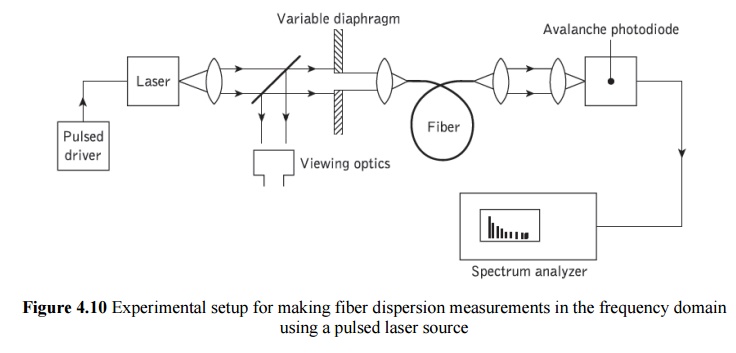
One of two frequency domain measurement techniques is generally used. The first utilizes a similar pulsed source to that employed for the time domain measurements shown in Figure 4.9. However, the sampling oscilloscope is replaced by a spectrum analyzer which takes the Fourier transform of the pulse in the time domain and hence displays its constituent frequency components. The experimental arrangement is illustrated in Figure 4.10. Comparison of the spectrum at the fiber output Po(w) with the spectrum at the fiber input Pi(w) provides the baseband frequency response for the fiber under test where:

The second technique involves launching a sinusoidally modulated optical signal at different selected frequencies using a sweep oscillator. Therefore the signal energy is concentrated in a very narrow frequency band in the baseband region, unlike the pulse measurement method where the signal energy is spread over the entire baseband region.