Dynamic Programming Code-Generation

Dynamic Programming Code-Generation

1 Contiguous Evaluation

2 The Dynamic Programming Algorithm

3 Exercises for Section 8.11

Algorithm 8.26 in Section 8.10 produces optimal code from an expression tree using an amount of time that is a linear function of the size of the tree. This procedure works for machines in which all computation is done in registers and in which instructions consist of an operator applied to two registers or to a register and a memory location.

An algorithm based on the principle of dynamic programming can be used to extend the class of machines for which optimal code can be generated from expression trees in linear time. The dynamic programming algorithm applies to a broad class of register machines with complex instruction sets.

The dynamic programming algorithm can be used to generate code for any machine with r interchangeable registers R0,R1, .. . , Rr—1 and load, store, and add instructions. For simplicity, we assume every instruction costs one unit, although the dynamic programming algorithm can easily be modified to work even if each instruction has its own cost.

1. Contiguous Evaluation

The dynamic programming algorithm partitions the problem of generating op-timal code for an expression into the subproblems of generating optimal code for the subexpressions of the given expression. As a simple example, consider an expression E of the form E1 + E₂. An optimal program for E is formed by combining optimal programs for E1 and E₂, in one or the other order, followed by code to evaluate the operator +. The subproblems of generating optimal code for E1 and E₂ are solved similarly.

An optimal program produced by the dynamic programming algorithm has an important property. It evaluates an expression E = E1 op E₂ "contigu-ously." We can appreciate what this means by looking at the syntax tree T for E:

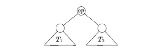
Here Ti  and T₂    are trees for E1  and E₂, respectively.

We say a program P evaluates a tree T contiguously if it first evaluates those subtrees of T that need to be computed into memory. Then, it evaluates the remainder of T either in the order Ti, T₂, and then the root, or in the order T₂, Ti, and then the root, in either case using the previously computed values from memory whenever necessary. As an example of noncontiguous evaluation, P might first evaluate part of Ti leaving the value in a register (instead of memory), next evaluate T₂, and then return to evaluate the rest of Ti.

For the register machine in this section, we can prove that given any mach-ine-language program P to evaluate an expression tree T, we can find an equiv-alent program P' such that

1. P' is of no higher cost than P,

    P' uses no more registers than P, and

    P' evaluates the tree contiguously.

This result implies that every expression tree can be evaluated optimally by a contiguous program.

By way of contrast, machines with even-odd register pairs do not always have optimal contiguous evaluations; the x86 architecture uses register pairs for mul-tiplication and division. For such machines, we can give examples of expression trees in which an optimal machine language program must first evaluate into a register a portion of the left subtree of the root, then a portion of the right subtree, then another part of the left subtree, then another part of the right, and so on. This type of oscillation is unnecessary for an optimal evaluation of any expression tree using the machine in this section.

The contiguous evaluation property defined above ensures that for any ex-pression tree T there always exists an optimal program that consists of optimal programs for subtrees of the root, followed by an instruction to evaluate the root. This property allows us to use a dynamic programming algorithm to generate an optimal program for T.

2. The Dynamic Programming Algorithm

The dynamic programming algorithm proceeds in three phases (suppose the target machine has r registers):

1. Compute bottom-up for each node n of the expression tree T an array C of costs, in which the zth component C[i] is the optimal cost of computing the subtree S rooted at n into a register, assuming i registers are available for the computation, for 1 < i < r.

2. Traverse T, using the cost vectors to determine which subtrees of T must be computed into memory.

Traverse each tree using the cost vectors and associated instructions to generate the final target code. The code for the subtrees computed into memory locations is generated first.

Each of these phases can be implemented to run in time linearly proportional to the size of the expression tree.

The cost of computing a node n includes whatever loads and stores are necessary to evaluate S in the given number of registers. It also includes the cost of computing the operator at the root of S. The zeroth component of the cost vector is the optimal cost of computing the subtree S into memory. The contiguous evaluation property ensures that an optimal program for S can be generated by considering combinations of optimal programs only for the subtrees of the root of S. This restriction reduces the number of cases that need to be considered.

In order to compute the costs C[i] at node n, we view the instructions as tree-rewriting rules, as in Section 8.9. Consider each template E that matches the input tree at node n. By examining the cost vectors at the corresponding descendants of n, determine the costs of evaluating the operands at the leaves of E. For those operands of E that are registers, consider all possible orders in which the corresponding subtrees of T can be evaluated into registers. In each ordering, the first subtree corresponding to a register operand can be evaluated using i available registers, the second using i -1 registers, and so on. To account for node n, add in the cost of the instruction associated with the template E. The value C[i] is then the minimum cost over all possible orders.

The cost vectors for the entire tree T can be computed bottom up in time linearly proportional to the number of nodes in T. It is convenient to store at each node the instruction used to achieve the best cost for C[i] for each value of i.  The smallest        cost in the vector for the root   of T gives the       minimum cost of evaluating T.                                     

Example 8.28: Consider a machine having two registers RO and Rl, and the following instructions, each of unit cost:

LD  Ri,  Kj    // Ri  =  Mj   

op  Ri,  Ri,  Ri  // Ri  =  Ri  Op  Rj

op  Ri,  Ri,  Mi  // Ri  =  Ri  Op  Kj

LD  Ri,  Ri    // Ri  =  Ri   

ST  Hi,  Ri    // Mi =  Rj   

In these instructions, Ri is either RO or Rl, and Mi is a memory location. The operator op corresponds to an arithmetic operators.

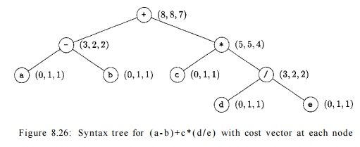
Let us apply the dynamic programming algorithm to generate optimal code for the syntax tree in Fig 8.26. In the first phase, we compute the cost vectors shown at each node. To illustrate this cost computation, consider the cost vector at the leaf a. C[0], the cost of computing a into memory, is 0 since it is already there. C[l], the cost of computing a into a register, is 1 since we can load it into a register with the instruction LD RO, a. C[2], the cost of loading a into a register with two registers available, is the same as that with one register available. The cost vector at leaf a is therefore (0,1,1).

Consider the cost vector at the root. We first determine the minimum cost of computing the root with one and two registers available. The machine instruction ADD RO, RO, M matches the root, because the root is labeled with the operator +. Using this instruction, the minimum cost of evaluating the root with one register available is the minimum cost of computing its right subtree into memory, plus the minimum cost of computing its left subtree into the register, plus 1 for the instruction. No other way exists. The cost vectors at the right and left children of the root show that the minimum cost of computing the root with one register available is 5 + 2 + 1 = 8.

Now consider the minimum cost of evaluating the root with two registers available. Three cases arise depending on which instruction is used to compute the root and in what order the left and right subtrees of the root are evaluated.

    Compute the left subtree with two registers available into register RO, compute the right subtree with one register available into register Rl, and use the instruction ADD RO, RO, Rl to compute the root. This sequence has cost 2 + 5 + 1 = 8.

   Compute the right subtree with two registers available into Rl, compute

the left subtree with one register available into RO, and use the instruction ADD RO, RO, Rl. This sequence has cost 4 + 2 + 1 = 7.

   Compute the right subtree into memory location M, compute the left sub-tree with two registers available into register RO, and use the instruction ADD RO, RO, M. This sequence has cost 5 + 2 + 1 = 8.

The second choice gives the minimum cost 7.

The minimum cost of computing the root into memory is determined by adding one to the minimum cost of computing the root with all registers avail-able; that is, we compute the root into a register and then store the result. The cost vector at the root is therefore (8,8,7).

From the cost vectors we can easily construct the code sequence by making a traversal of the tree. From the tree in Fig. 8.26, assuming two registers are available, an optimal code sequence is

LD  RO,  c    // RO  =  c

LD  Rl,  d    // Rl  =  d

DIV  Rl,  Rl,  e  // Rl  =  Rl  / e

MUL  RO,  RO,  Rl  // RO  =  RO  * Rl

LD  Rl,  a    // Rl  =  a

SUB  Rl,  Rl,  b  // Rl =  Rl  - b

ADD  Rl,  Rl,  RO  // Rl  =  Rl  +  RO

Dynamic programming techniques have been used in a number of compilers, including the second version of the portable C compiler, PCC2 . The technique facilitates retargeting because of the applicability of the dynamic programming technique to a broad class of machines.

3. Exercises for Section 8.11

Exercise 8 . 1 1 . 1 : Augment the tree-rewriting scheme in Fig. 8.20 with costs, and use dynamic programming and tree matching to generate code for the statements in Exercise 8.9.1.

Exercise 8.11.2 : How would you extend dynamic programming to do optimal code generation on dags?

Summary of Chapter 8

Code generation is the final phase of a compiler. The code generator maps the intermediate representation produced by the front end, or if there is a code optimization phase by the code optimizer, into the target program.

•  Instruction  selection  is  the  process  of choosing  target-language  instructions for each IR statement.        

•  Register  allocation  is  the  process  of deciding  which  IR  values  to  keep in registers.  Graph coloring is an effective technique for doing register allocation in compilers.         

•  Register  assignment  is  the  process  of deciding  which  register should  hold a given  IR  value.             

  A retargetable compiler is one that can generate code for multiple instruc-tion sets.

  A  virtual machine is an interpreter for a bytecode intermediate language produced by languages such as Java and C # .

 A CISC machine is typically a two-address machine with relatively few registers, several register classes, and variable-length instructions with complex addressing modes.

  A RISC machine is typically a three-address machine with many registers in which operations are done in registers.

  A basic block is a maximal sequence of consecutive three-address state-ments in which flow of control can only enter at the first statement of the block and leave at the last statement without halting or branching except possibly at the last statement in the basic block.

  A flow graph is a graphical representation of a program in which the nodes of the graph are basic blocks and the edges of the graph show how control can flow among the blocks.

 A loop in a flow graph is a strongly connected region with a single entry point called the loop header.

  A DAG representation of a basic block is a directed acyclic graph in which the nodes of the DAG represent the statements within the block and each child of a node corresponds to the statement that is the last definition of an operand used in the statement.

• Peephole optimizations are local code-improving transformations that can be applied to a program, usually through a sliding window.

*  Instruction  selection  can  be  done  by  a  tree-rewriting  process  in  which tree patterns corresponding to machine instructions are used to tile a syntax tree. We can associate costs with the tree-rewriting rules and apply dynamic programming to obtain an optimal tiling for useful classes of machines and expressions.

An Ershov number tells how many registers are needed to evaluate an expression without storing any temporaries.

• Spill code is an instruction sequence that stores a value in a register into memory in order to make room to hold another value in that register.