Basic Blocks and Flow Graphs

Basic Blocks and Flow Graphs

1 Basic Blocks

2 Next-Use Information

3 Flow Graphs

4 Representation of Flow Graphs

5 Loops

6 Exercises for Section 8.4

This section introduces a graph representation of intermediate code that is help-ful for discussing code generation even if the graph is not constructed explicitly by a code-generation algorithm. Code generation benefits from context. We can do a better job of register allocation if we know how values are defined and used, as we shall see in Section 8.8. We can do a better job of instruction selection by looking at sequences of three-address statements, as we shall see in Section 8.9.

The representation is constructed as follows:

  Partition the intermediate code into basic blocks, which are maximal se-quences of consecutive three-address instructions with the properties that

           The flow of control can only enter the basic block through the first instruction in the block. That is, there are no jumps into the middle of the block.

            Control will leave the block without halting or branching, except possibly at the last instruction in the block.

The basic blocks become the nodes of a flow graph, whose edges indicate which blocks can follow which other blocks.

The Effect of Interrupts

The notion that control, once it reaches the beginning of a basic block is certain to continue through to the end requires a bit of thought. There are many reasons why an interrupt, not reflected explicitly in the code, could cause control to leave the block, perhaps never to return. For example, an instruction like x  =  y / z appears not to affect control flow, but if z is 0 it could actually cause the program to abort.

We shall not worry about such possibilities. The reason is as follows. The purpose of constructing basic blocks is to optimize the code. Gener-ally, when an interrupt occurs, either it will be handled and control will come back to the instruction that caused the interrupt, as if control had never deviated, or the program will halt with an error. In the latter case, it doesn't matter how we optimized the code, even if we depended on control reaching the end of the basic block, because the program didn't produce its intended result anyway.

Starting in Chapter 9, we discuss transformations on flow graphs that turn the original intermediate code into "optimized" intermediate code from which better target code can be generated. The "optimized" intermediate code is turned into machine code using the code-generation techniques in this chapter.

1. Basic Blocks

Our first job is to partition a sequence of three-address instructions into basic blocks. We begin a new basic block with the first instruction and keep adding instructions until we meet either a jump, a conditional jump, or a label on the following instruction. In the absence of jumps and labels, control proceeds sequentially from one instruction to the next. This idea is formalized in the following algorithm.

A l g o r i t h m 8.5 :  Partitioning three-address instructions into basic blocks.

INPUT: A sequence of three-address instructions.

OUTPUT: A list of the basic blocks for that sequence in which each instruction is assigned to exactly one basic block.

METHOD: First, we determine those instructions in the intermediate code that are leaders, that is, the first instructions in some basic block. The instruction just past the end of the intermediate program is not included as a leader. The rules for finding leaders are:

1. The first three-address instruction in the intermediate code is a leader.

2. Any instruction that is the target of a conditional or unconditional jump is a leader.

    Any instruction that immediately follows a conditional or unconditional jump is a leader.

Then, for each leader, its basic block consists of itself and all instructions up to but not including the next leader or the end of the intermediate program.

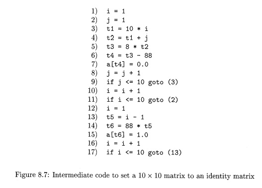
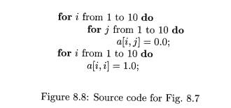
Example 8 . 6 : The intermediate code in Fig. 8.7 turns a 10 x 10 matrix a into an identity matrix. Although it is not important where this code comes from, it might be the translation of the pseudocode in Fig. 8.8. In generating the intermediate code, we have assumed that the real-valued array elements take 8 bytes each, and that the matrix a is stored in row-major form.

First, instruction 1 is a leader by rule (1) of Algorithm 8.5. To find the other leaders, we first need to find the jumps. In this example, there are three jumps, all conditional, at instructions 9, 11, and 17. By rule (2), the targets of these jumps are leaders; they are instructions 3, 2, and 13, respectively. Then, by rule (3), each instruction following a jump is a leader; those are instructions 10 and 12. Note that no instruction follows 17 in this code, but if there were code following, the 18th instruction would also be a leader.

We conclude that the leaders are instructions 1, 2, 3, 10, 12, and 13. The basic block of each leader contains all the instructions from itself until just before the next leader. Thus, the basic block of 1 is just 1, for leader 2 the block is just 2. Leader 3, however, has a basic block consisting of instructions 3 through 9, inclusive. Instruction 10's block is 10 and 11; instruction 12's block is just 12, and instruction 13's block is 13 through 17. •

2. Next-Use Information

Knowing when the value of a variable will be used next is essential for generating good code. If the value of a variable that is currently in a register will never be referenced subsequently, then that register can be assigned to another variable.

The use of a name in a three-address statement is defined as follows. Suppose three-address statement i assigns a value to x. If statement j has x as an operand, and control can flow from statement i to j along a path that has no intervening assignments to x, then we say statement j uses the value of x computed at statement i. We further say that x is live at statement i.

We wish to determine for each three-address statement x = y + z what the next uses of x, y, and z are. For the present, we do not concern ourselves with uses outside the basic block containing this three-address statement.

Our algorithm to determine liveness and next-use information makes a back-ward pass over each basic block. We store the information in the symbol table. We can easily scan a stream of three-address statements to find the ends of ba-sic blocks as in Algorithm 8.5. Since procedures can have arbitrary side effects, we assume for convenience that each procedure call starts a new basic block.

Algorithm 8 . 7 : Determining the liveness and next-use information for each statement in a basic block.

INPUT: A basic block B of three-address statements. We assume that the symbol table initially shows all nontemporary variables in B as being live on exit.

OUTPUT: At each statement i: x = y + z in B, we attach to i the liveness and next-use information of x, y, and z.

METHOD: We start at the last statement in B and scan backwards to the beginning of B. At each statement i: x = y + z in B, we do the following:

1. Attach to statement i the information currently found in the symbol table regarding the next use and liveness of x, y, and y.

2. In the symbol table, set x to "not live"  and "no next use."

3. In the symbol table, set y and z to "live" and the next uses of y and z to  i.  

Here we have used + as a symbol representing any operator. If the three-address statement i is of the form x = + y or x = y, the steps are the same as above, ignoring z. Note that the order of steps (2) and (3) may not be interchanged because x may be y or z. •

3. Flow Graphs

Once an intermediate-code program is partitioned into basic blocks, we repre-sent the flow of control between them by a flow graph. The nodes of the flow graph are the basic blocks. There is an edge from block B to block C if and only if it is possible for the first instruction in block C to immediately follow the last instruction in block B. There are two ways that such an edge could be justified:

 There is a conditional or unconditional jump from the end of B to the beginning of C.

C immediately follows B in the original order of the three-address instruc-tions, and B does not end in an unconditional jump .

We say that  B is a predecessor of C,  and C is a successor of B.

Often we add two nodes, called the entry and exit, that do not correspond to executable intermediate instructions. There is an edge from the entry to the first executable node of the flow graph, that is, to the basic block that comes from the first instruction of the intermediate code. There is an edge to the exit from any basic block that contains an instruction that could be the last executed instruction of the program. If the final instruction of the program is not an unconditional jump, then the block containing the final instruction of the program is one predecessor of the exit, but so is any basic block that has a jump to code that is not part of the program.

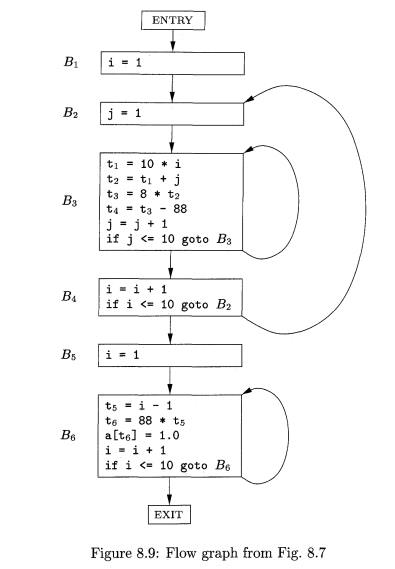
Example 8 . 8 :  The set of basic blocks constructed in Example 8.6 yields the flow graph of Fig.  8.9. The entry points to basic block B1,  since B1 contains the first instruction of the program.  The only successor of B1  is B2, because B1  does not end in an unconditional jump,  and the leader of B2 immediately follows the  end of B1.

Block B3   has two successors.  One is itself, because the leader of B3, instruction 3, is the target of the conditional jump at the end of £3, instruction 9. The other successor is B4, because control can fall through the conditional jump at the end of B3 and next enter the leader of B±.

Only B6 points to the exit of the flow graph, since the only way to get to code that follows the program from which we constructed the flow graph is to fall through the conditional jump that ends B₆.

4. Representation of Flow Graphs

First, note from Fig. 8.9 that in the flow graph, it is normal to replace the jumps to instruction numbers or labels by jumps to basic blocks. Recall that every conditional or unconditional jump is to the leader of some basic block, and it is to this block that the jump will now refer.

The reason for this change is that after constructing the flow graph, it is common to make substantial changes to the instructions in the various basic blocks.  If jumps were to instructions, we would have to fix the targets of the jumps every time one of the target instructions was changed.

Flow graphs, being quite ordinary graphs, can be represented by any of the data structures appropriate for graphs. The content of nodes (basic blocks) need their own representation. We might represent the content of a node by a pointer to the leader in the array of three-address instructions, together with a count of the number of instructions or a second pointer to the last instruction. However, since we may be changing the number of instructions in a basic block frequently, it is likely to be more efficient to create a linked list of instructions for each basic block.

5. Loops

Programming-language constructs like while-statements, do-while-statements, and for-statements naturally give rise to loops in programs. Since virtually every program spends most of its time in executing its loops, it is especially important for a compiler to generate good code for loops. Many code transformations depend upon the identification of "loops" in a flow graph. We say that a set of nodes L in a flow graph is a loop if

   There is a node in L called the loop entry with the property that no other node in L has a predecessor outside L. That is, every path from the entry

of the entire flow graph to any node in L goes through the loop entry.

   Every node in L has a nonempty path, completely within L, to the entry of L.

Example 8 . 9 :  The flow graph of Fig. 8.9 has three loops:

1. B3 by itself.   

2. B6 by itself.   

3. {B2,  B3, B4}.   

The first two are single nodes with an edge to the node itself.  For instance, B3    forms a loop with B3 as its entry.  Note that the second requirement for a loop is that there be a nonempty path from B3 to itself. Thus, a single node like B2, which does not have an edge B2 ->• B2, is not a loop, since there is no nonempty  path  from B2 to  itself within {B2}. 

The third loop, L = {B2, B3, B4}, has B2 as its loop entry.  Note that among these three nodes, only B2 has a predecessor, Bi, that is not in L. Further, each of the three nodes has a nonempty path to B2    staying within L. For instance, B2    has the path B2    ->• B3 ->• B4    -> B2.

6. Exercises for Section 8.4

Exercise 8 . 4 . 1 :  Figure 8.10 is a simple matrix-multiplication program.

a) Translate the program into three-address statements of the type we have been using in this section. Assume the matrix entries are numbers that require 8 bytes, and that matrices are stored in row-major order.

    Construct the flow graph for your code from (a).

    Identify the loops in your flow graph from (b).

for (i=0; i<n; i++)

for (j=0; j<n; j++) c[i] [j] = 0.0;

for (i=0; i<n; i++)

for (j=0; j<n; j++)

for (k=0; k<n; k++)

c[i][j]  = c[i][j]  + a[i][k]*b[k][j];

Figure 8.10: A matrix-multiplication algorithm

Exercise 8.4.2: Figure 8.11 is code to count the number of primes from 2 to n, using the sieve method on a suitably large array a.  That is, a[i] is TRUE at the end only if there is no prime Vi or less that evenly divides i.  We initialize all a[i] to TRUE and then set a1j] to FALSE if we find a divisor of j.

     Translate the program into three-address statements of the type we have been using in this section. Assume integers require 4 bytes.

b)  Construct the flow graph for your code from   (a).

c) Identify the loops in your flow graph from (b).

for (i=2; i<=n; i++) a[i] = TRUE;

count = 0;

s  =  sqrt(n);

for  (i=2;  i<=s;         i++)

if  (a[i])  /*  i has been found to be a prime */ {

count++;

for  (j=2*i;  j<=n;  j  = j+i)

a[j]  = FALSE;  /* no multiple of  i  is a prime */

}

Figure 8.11: Code to sieve for primes