D.C and A.C Bridges

D.C & A.C Bridges

Bridge circuits are used very commonly as a variable conversion element in measurement systems and produce an output in the form of a voltage level that changes as the measured physical quantity changes. They provide an accurate method of measuring resistance, inductance and capacitance values, and enable the detection of very small changes in these quantities about a nominal value. They are of immense importance in measurement system technology because so many transducers measuring physical quantities have an output that is expressed as a change in resistance, inductance or capacitance. The displacement-measuring strain gauge, which has a varying resistance output, is but one example of this class of transducers. Normally, excitation of the bridge is by a d.c. voltage for resistance measurement and by an a.c. voltage for inductance or capacitance measurement. Both null and deflection types of bridge exist, and, in a like manner to instruments in general, null types are mainly employed for calibration purposes and deflection types are used within closed-loop automatic control schemes.

Null-type, d.c. bridge (Wheatstone bridge)

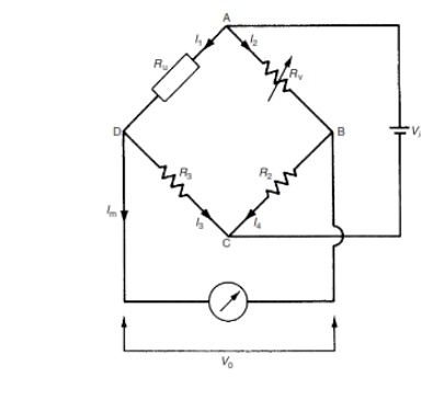
A null-type bridge with d.c. excitation, commonly known as a Wheatstone bridge, has the form shown in Figure 7.1. The four arms of the bridge consist of the unknown resistance Ru, two equal value resistors R2 and R3 and a variable resistor Rv (usually a decade resistance box). A d.c. voltage Vi is applied across the points AC and the resistance Rv is varied until the voltage measured across points BD is zero. This null point is usually measured with a high sensitivity galvanometer.

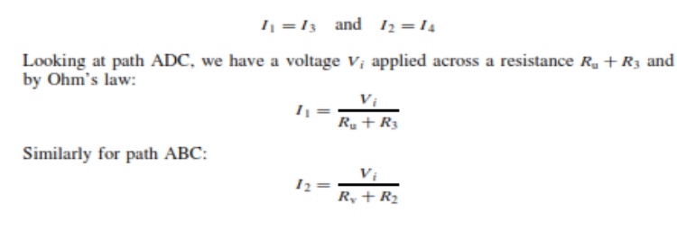
To analyses the Whetstone bridge, define the current flowing in each arm to be I1 . . . I4 as shown in Figure 7.1. Normally, if a high impedance voltage-measuring instrument is used, the current Im drawn by the measuring instrument will be very small and can be approximated to zero. If this assumption is made, then, for Im D 0:

I1 =I3 and    I2 =I4

Deflection-type d.c. bridge

A deflection-type bridge with d.c. excitation is shown in Figure 7.2. This differs from the Wheatstone bridge mainly in that the variable resistance Rvis replaced by a fixed resistance R1 of the same value as the nominal value of the unknown resistance Ru . As the resistance Ru changes, so the output voltage V0 varies, and this relationship between V0 and Ru must be calculated.

This relationship is simplified if we again assume that a high impedance voltage measuring instrument is used and the current drawn by it, Im , can be approximated to zero. (The case when this assumption does not hold is covered later in this section.) The analysis is then exactly the same as for the preceding example of the Wheatstone bridge, except that Rv is replaced by R1. Thus, from equation (7.1), we have:

V0= Vi * ( Ru / Ru + R3)- (  R1 / R1+ R2)

When Ru is at its nominal value, i.e. for Ru D R1, it is clear that V0 D0 (since R2 D R3). For other values of Ru, V0 has negative and positive values that vary in a non-linear way with Ru.

A.C bridges

Bridges with a.c. excitation are used to measure unknown impedances. As for d.c. bridges, both null and deflection types exist, with null types being generally reserved for calibration duties.

Null-type impedance bridge

A typical null-type impedance bridge is shown in Figure 7.7. The null point can be conveniently detected by monitoring the output with a pair of headphones connected via an operational amplifier across the points BD. This is a much cheaper method of null detection than the application of an expensive galvanometer that is required for a d.c. Wheatstone bridge.

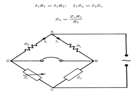
If Zu i s capacitive, i.e. Zu D 1/jωCu, then Zv m u s t consist of a variable capacitance box, which is readily available. If Zu is inductive, then Zu D Ru C jωLu .

Notice that the expression for Zu as an inductive impedance has a resistive term in it because it is impossible to realize a pure inductor. An inductor coil always has a resistive component, though this is made as small as possible by designing the coil to have a high Q factor (Q factor is the ratio inductance/resistance). Therefore, Zv must consist of a variable-resistance box and a variable-inductance box. However, the latter are not readily available because it is difficult and hence expensive to manufacture a set of fixed value inductors to make up a variable-inductance box. For this reason, an alternative kind of null-type bridge circuit, known as the Maxwell Bridge, is commonly used to measure unknown inductances.

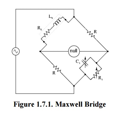
Maxwell bridge

Definition

A Maxwell bridge (in long form, a Maxwell-Wien bridge) is a type of Wheatstone bridge used to measure an unknown inductance (usually of low Q value) in terms of calibrated resistance and capacitance. It is a real product bridge.

The maxwell bridge is used to measure unknown inductance in terms of calibrated resistance and capacitance. Calibration-grade inductors are more difficult to manufacture than capacitors of similar precision, and so the use of a simple "symmetrical" inductance bridge is not always practical.

Circuit Diagram

Explanation

With reference to the picture, in a typical application R1 and R4 are known fixed entities, and R2 and C2 are known variable entities.

R2 and C2 are adjusted until the bridge is balanced.R3 and L3 can then be calculated based on the values of the other components:

As shown in Figure, one arm of the Maxwell bridge consists of a capacitor in parallel with a resistor (C1 and R2) and another arm consists of an inductor L1 in series with a resistor (L1 and R4). The other two arms just consist of a resistor each (R1 and R3).

The values of R1 and R3 are known, and R2 and C1 are both adjustable. The unknown values are those of L1 and R4.

 Like other bridge circuits, the measuring ability of a Maxwell Bridge depends on 'Balancing' the circuit.

Balancing the circuit in Figure 1 means adjusting C1 and R2 until the current through the bridge between points A and B becomes zero. This happens when the voltages at points A and B are equal.

Mathematically,

Z1 = R2 + 1/ (2πfC1); while Z2 = R4 + 2πfL1.

(R2 + 1/ (2πfC1)) / R1 = R3 / [R4 + 2πfL1];

or

R1R3 = [R2 + 1/ (2πfC1)] [R4 + 2πfL1]

To avoid the difficulties associated with determining the precise value of a variable capacitance, sometimes a fixed-value capacitor will be installed and more than one resistor will be made variable.

The additional complexity of using a Maxwell bridge over simpler bridge types is warranted in circumstances where either the mutual inductance between the load and the known bridge entities, or stray electromagnetic interference, distorts the measurement results.

The capacitive reactance in the bridge will exactly oppose the inductive reactance of the load when the bridge is balanced, allowing the load's resistance and reactance to be reliably determined.

Advantages:

The frequency does not appear

Wide range of inductance

Disadvantages:

Limited measurement

It requires variable standard capacitor

SCHERING BRIDGE

Definition

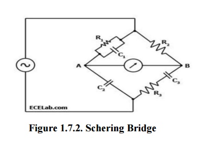
A  Schering Bridge is a   bridge circuit used for measuring an  unknown  electrical capacitance and its dissipation factor. The dissipation factor of a capacitor is the the ratio of its resistance  to its  capacitive  reactance.  The  Schering Bridge is  basically a four-arm alternating-

current (AC) bridge circuit whose measurement depends on balancing the loads on its arms   Figure 1 below shows a diagram of the Schering Bridge.

Diagram

Explanation

In the Schering Bridge above, the resistance values of resistors R1 and R2 are known, while the resistance value of resistor R3 is unknown.

The capacitance values of C1 and C2 are also known, while the capacitance of C3 is the value being measured.

To measure R3 and C3, the values of C2 and R2 are fixed, while the values of R1 and C1 are adjusted until the current through the ammeter between points A and B becomes zero.

This happens when the voltages at points A and B are equal, in which case the bridge is said to be 'balanced'.

When the bridge is balanced, Z1/C2 = R2/Z3, where Z1 is the impedance of R1 in parallel with C1 and Z3 is the impedance of R3 in series with C3.

In an AC circuit that has a capacitor, the capacitor contributes a capacitive reactance to the impedance.

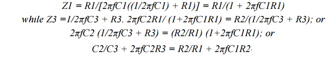
When the bridge is balanced, the negative and positive reactive components are equal and cancel out, so

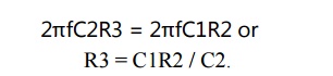
Similarly, when the bridge is balanced, the purely resistive components are equal, 

so C2/C3 = R2/R1 or C3 = R1C2 / R2.

Note that the balancing of a Schering Bridge is independent of frequency.

Advantages:

Balance equation is independent of frequency

Used for measuring the insulating properties of electrical cables and equipment’s

HAY BRIDGE

Definition

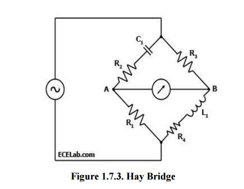
A Hay Bridge is an AC bridge circuit used for measuring an unknown inductance by balancing the loads of its four arms, one of which contains the unknown inductance. One of the arms of a Hay Bridge has a capacitor of known characteristics, which is the principal component used for determining the unknown inductance value. Figure 1 below shows a diagram of the Hay Bridge.

Explanation

As shown in Figure 1, one arm of the Hay bridge consists of a capacitor in series with a resistor (C1 and R2) and another arm consists of an inductor L1in series with a resistor (L1 and R4).

The other two arms simply contain a resistor each (R1 and R3). The values of R1and R3 are known, and R2 and C1 are both adjustable.

The unknown values are those of L1 and R4.

Like other bridge circuits, the measuring ability of a Hay Bridge depends on 'balancing' the circuit.

Balancing the circuit in Figure 1 means adjusting R2 and C1 until the current through the ammeter between points A and B becomes zero. This happens when the voltages at points A and B are equal.

Diagram

When the Hay Bridge is balanced, it follows that Z1/R1 = R3/Z2 wherein Z1 is the impedance of the arm containing C1 and R2 while Z2 is the impedance of the arm containing L1 and R4.

Thus, Z1 = R2 + 1/(2πfC) while Z2 = R4 + 2πfL1.

[R2 + 1/(2πfC1)]  / R1 = R3 / [R4 + 2πfL1]; or

[R4 + 2πfL1] = R3R1 / [R2 + 1/(2πfC1)]; or

R3R1 = R2R4 + 2πfL1R2 + R4/2πfC1 + L1/C1.

When the bridge is balanced, the reactive components are equal, so

2πfL1R2 = R4/2πfC1, or R4 = (2πf) 2L1R2C1.

Substituting R4, one comes up with the following equation:

R3R1 = (R2+1/2πfC1) ((2πf) 2L1R2C1) + 2πfL1R2 + L1/C1; or

L1 = R3R1C1 / (2πf) 2R22C12 + 4πfC1R2 + 1);

L1 = R3R1C1 / [1 + (2πfR2C1)2]

After dropping the reactive components of the equation since the bridge is

Thus, the equations for L1 and R4 for the Hay Bridge in Figure 1 when it is balanced are:

L1 = R3R1C1 / [1 + (2πfR2C1)2]; and

R4 = (2πfC1)2R2R3R1 / [1 + (2πfR2C1)2]

Advantages:

Simple expression

Disadvantages:

It is not suited for measurement of coil

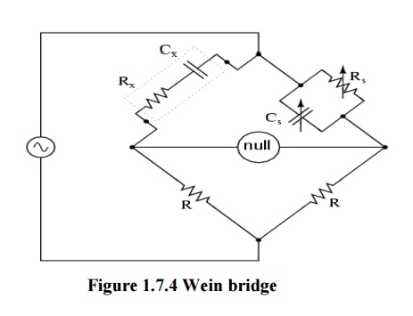
WIEN BRIDGE:

Definition

A Wien bridge oscillator is a type of electronic oscillator that generates sine waves. It can generate a large range of frequencies. The circuit is based on an electrical network originally developed by Max Wien in 1891. Wien did not have a means of developing electronic gain so a workable oscillator could not be realized. The modern circuit is derived from William Hewlett's 1939 Stanford University master's degree thesis. Hewlett, along with David Packard co-founded Hewlett-Packard. Their first product was the HP 200A, a precision sine wave oscillator based on the Wien bridge. The 200A was one of the first instruments to produce such low distortion.

Diagram

Amplitude stabilization:

The key to Hewlett's low distortion oscillator is effective amplitude stabilization.

The amplitude of electronic oscillators tends to increase until clipping or other gain limitation is reached. This leads to high harmonic distortion, which is often undesirable.

Hewlett used an incandescent bulb as a positive temperature coefficient (PTC) thermistor in the oscillator feedback path to limit the gain.

The resistance of light bulbs and similar heating elements increases as their temperature increases.

If the oscillation frequency is significantly higher than the thermal time constant of the heating element, the radiated power is proportional to the oscillator power.

Since heating elements are close to black body radiators, they follow the Stefan-Boltzmann law.

The radiated power is proportional to T4, so resistance increases at a greater rate than amplitude.

If the gain is inversely proportional to the oscillation amplitude, the oscillator gain stage reaches a steady state and operates as a near ideal class A amplifier, achieving very low distortion at the frequency of interest.

At lower frequencies the time period of the oscillator approaches the thermal time constant of the thermistor element and the output distortion starts to rise significantly. Light bulbs have their disadvantages when used as gain control elements in Wien bridge oscillators, most notably a very high sensitivity to vibration due to the bulb's micro phonic nature amplitude modulating the oscillator output, and a limitation in high frequency response due to the inductive nature of the coiled filament.

Modern Distortion as low as 0.0008% (-100 dB) can be achieved with only modest improvements to Hewlett's original circuit.

Wien bridge oscillators that use thermistors also exhibit "amplitude bounce" when the oscillator frequency is changed. This is due to the low damping factor and long time constant of the crude control loop, and disturbances cause the output amplitude to exhibit a decaying sinusoidal response.

This can be used as a rough figure of merit, as the greater the amplitude bounce after a disturbance, the lower the output distortion under steady state conditions.

Analysis:

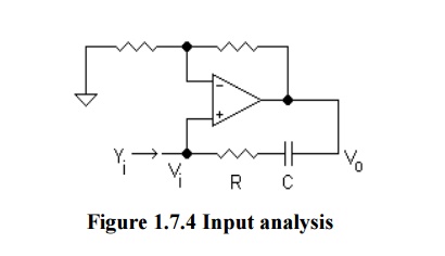
Input admittance analysis

If Av is greater than 1, the input admittance is a negative resistance in parallel with an inductance.

If a resistor is placed in parallel with the amplifier input, it will cancel some of the negative resistance. If the net resistance is negative, amplitude will grow until clipping occurs.

If a resistance is added in parallel with exactly the value of R, the net resistance will be infinite and the circuit can sustain stable oscillation at any amplitude allowed by the amplifier.

Advantages:

Frequency sensitive

Supply voltage is purely sinusoidal