Creating Formulae - OpenOffice Calc

Creating Formulae

After entering the data in worksheet, you can perform calculations on the data in the worksheet. In order to create formulae, you first need to know the syntax that describes the format for specifying a formula.

In Calc, you can enter formulas in two methods, either directly into the cell or at the input line. Formula in Calc may start with equal (=) or plus(+) or minus(–) sign followed by a combination of values, operators and cell references. But, as a general practice, all formulas should start with an equal sign. If any formula starts with a + or –, the values will be considered as positive or negative respectively.

Operators

Operators are symbols for doing some mathematical, statistical and logical calculations. Combination of values, operators and cell references is called as “Expression”. Calc supports a variety of operators which are categorized as:

(1) Arithmetic Opertors

(2) Relational Operators

(3) Reference Operators

(4) Text Operator

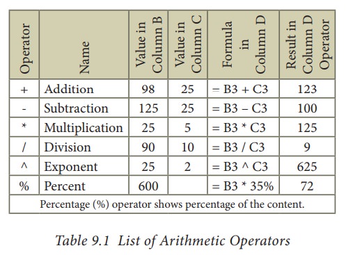
1. Arithmetic Operators

Arithmetic operators are symbols for performing simple arithmetic operations such as addition, subtraction, multiplication, division etc., These operators return a numerical result.

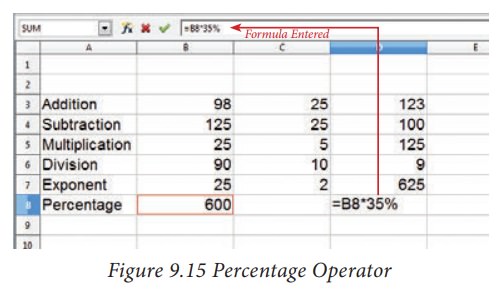
Formula bar shows the formula what the user had entered. But, the cell shows the resulted value (Figure 9.15).

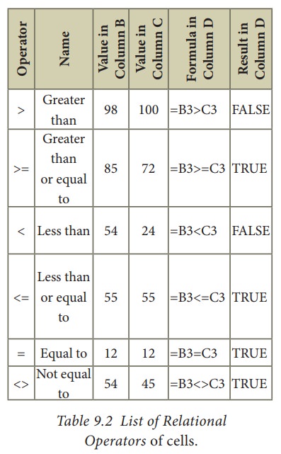
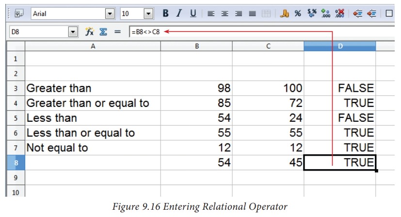
2. Relational Operators

Relational operators are symbols used for comparing two values such as greater than, less than, equal to etc. The relational operators are also called as "Comparative operators". These operators return either a True or a False.

3. Reference Operator

Reference operators are used to refer cell ranges. A continuous group of cells is called as “Range”. There are three types of reference operators that are used to refer cells in calc; they are Range Reference Operator, (2) Range Concatenation (3) Intersection Operator.

Range Reference Operator

Colon (:) is the range reference operator. It is used to group a range of cells. An expression using a range operator has the following syntax:

reference left : reference right

where reference left is the starting cell address of a linear group of cells or upper left corner address of a rectangular group Reference right is the last cell address of a linear group or lower right corner address of a rectangular group of cell.

Example:

(i) Linear group of cells A1, A2,A3,A4,A5 is referred as A1:A5

(ii) Rectangular group of cells A2, A3, A4, ….. B2, B3, B4,….D5, D6 is referred as A2:D6 (Refer Figure 7.17)

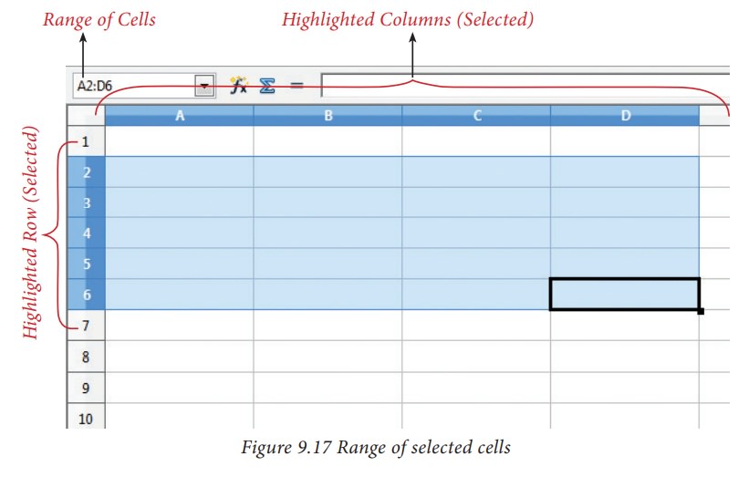
Name box shows the reference A2:D6 corresponding to the cells included in the drag operation with the mouse to highlight the range.

Reference concatenation operator:

Concatenation means joining together. Tilde (~) symbol is used as a concatenation operator in calc. An expression using a concatenation operator has the following syntax:

reference left ~ reference right

Example:

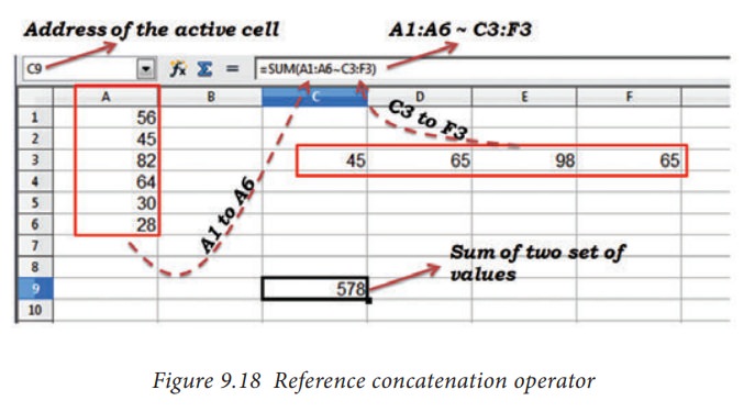
If you want to find the sum of the values from A1 to A6 and C3 to F3. The formula is =SUM(A1:A6 ~ C3:F3)

SUM is a function to find the sum of a group of values. (Refer Figure 9.18)

Intersection Operator:

Intersection operator is used to join two set of groups. It is very similar to Range concatenation operator. The intersection operator is represented by an exclamation

reference left ! reference right

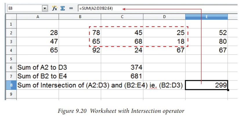
Example: (A2:D3 ! B2:E4)

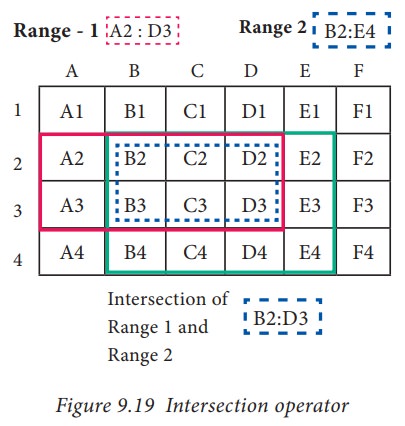
The result of (A2:D3 ! B2:E4) is referred by the range B2:D3, because these cells are both inside A2:D3 and B2:E4 (Refer Figure 9.19 and 9.20).

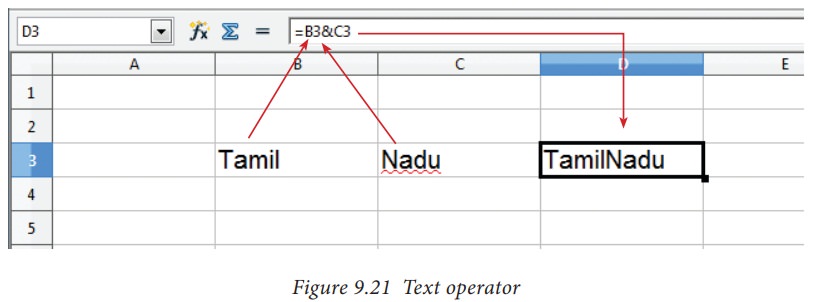
4. Text Operator:

In Calc, “&” is a text operator which is used to combine two or more text. Joining two different texts is also known as “Text Concatenation” (Refer Figure 9.21). An expression using the text operator has the following syntax:

text reference1 & text reference2

When arithmetic operators are used in a formula, Calc calculates the results using the rule of precedence followed in Mathematics. The order is:

I. Exponentiation ( ^ )

II. Negation ( - )

III. Multiplication and Division ( *, /)

IV. Addition and Subtraction (+, -)

Here is an example to illustrate how to create a formula:

Illustration 1:

Create a Marks worksheet with the following data:

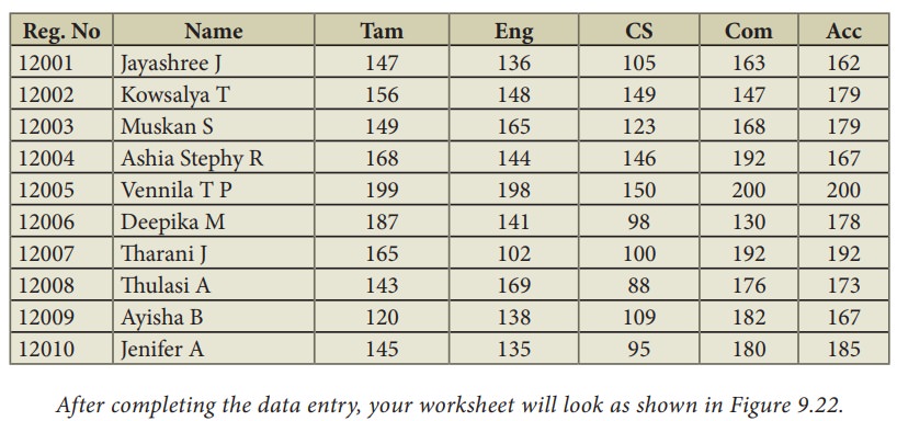
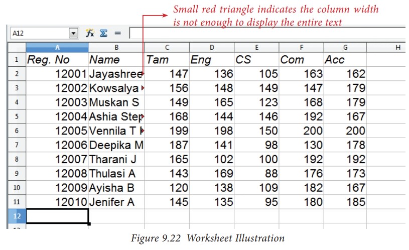
After completing the data entry, your worksheet will look as shown in Figure 9.22.

Construction of formula

To construct a formula, follow the steps below:

• Cell pointer should be in the cell in which you want to display the result.

• Formula should begin with an = sign.

• In a formula, use only cell reference (cell address) instead of the actual values within the cells.

• While constructing a formula, BODMAS rule should be kept in mind.

• eneral Syntax of constructing a formula is: = cell reference1 <operator> cell reference2 <operator> ……………….

• Cell references are of two types (i) Relative cell reference (ii) Absolute Cell reference.

• If you refer cell addresses directly while constructing formulae, it is called as “Relative Cell addressing”.

• Examples of Relative Cell addressing:

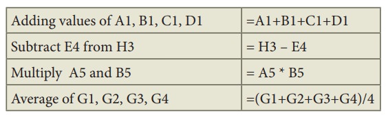
Adding values of A1, B1, C1, D1 =A1+B1+C1+D1

Subtract E4 from H3 = H3 – E4

Multiply A5 and B5 = A5 * B5

Average of G1, G2, G3, G4 =(G1+G2+G3+G4)/4

• In the above table, all cell references are “Relative cell addressing:”.

• While writing a formula, if you use the $ symbol in front of a column name and row number, it will become an “Absolute Cell addressing”.

• Examples of Absolute cell addressing:

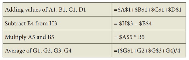
Adding values of A1, B1, C1, D1 =$A$1+$B$1+$C$1+$D$1

Subtract E4 from H3 = $H$3 – $E$4

Multiply A5 and B5 = $A$5 * B5

Average of G1, G2, G3, G4 =($G$1+G2+$G$3+G4)/4

• In an expression, all cells need not necessarily be relative or absolute. You can mix both type of references.

• The following section explains the use of relative cell addressing. About “Absolute cell addressing”, you will be learn later in this chapter.

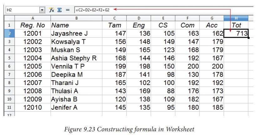
Finding Total to the above Illustration:

• Move the cell pointer to H2 (Total column)

• Type the following formula; after entering the formula, press “Enter” key = C2+D2+E2+F2+G2 (Refere Figure 9.25)

• Now, you will get the sum of all the values of C2, D2, E2, F2 and G2

• The above-mentioned formula clearly stated that, how worksheets are working with cells.

• While referring to the cell addresses in a formula, the spreadsheet reads the value inside the cell that you refer. This is a good practice of constructing a formula. Because, if you change any value, the spreadsheet recalculates with that new value.

After entering a formula the result is display as in Figure 9.23