Central Limit Theorem

CENTRAL LIMIT THEOREM:

In probability theory, the central limit theorem (CLT) states that, given certain conditions, the arithmetic mean of a sufficiently large number of iterates of independent random variables, each with a well-defined expected value and well-defined variance, will be approximately normally distributed.

The Central Limit Theorem describes the characteristics of the "population of the means" which has been created from the means of an infinite number of random population samples of size (N), all of them drawn from a given "parent population". The Central Limit Theorem predicts that regardless of the distribution of the parent population:

[1] The mean of the population of means is always equal to the mean of the parent population from which the population samples were drawn.

[2] The standard deviation of the population of means is always equal to the standard deviation of the parent population divided by the square root of the sample size (N).

[3] The distribution of means will increasingly approximate a normal distribution as the size N of samples increases.

A consequence of Central Limit Theorem is that if we average measurements of a particular quantity, the distribution of our average tends toward a normal one. In addition, if a measured variable is actually a combination of several other uncorrelated variables, all of them "contaminated" with a random error of any distribution, our measurements tend to be contaminated with a random error that is normally distributed as the number of these variables increases.Thus, the Central Limit Theorem explains the ubiquity of the famous bell-shaped "Normal distribution" (or "Gaussian distribution") in the measurements domain.

Examples:

•   Uniform distribution

•   Triangular distribution

•   1/X distribution

•   Parabolic distribution

•   CLT Summary

•   more statistical fine-print

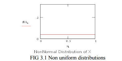
The uniform distribution on the left is obviously non-Normal. Call that the parent distribution.

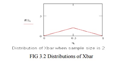
To compute an average, Xbar, two samples are drawn, at random, from the parent distribution and averaged. Then another sample of two is drawn and another value of Xbar computed. This process is repeated, over and over, and averages of two are computed. The distribution of averages of two is shown on the left.

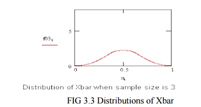
Repeatedly taking three from the parent distribution, and computing the averages, produce the probability density on the left.