CPU Scheduling

CPU SCHEDULING

ü               Basic Concepts

   Almost all programs have some alternating cycle of CPU number crunching and waiting for I/O of some kind. ( Even a simple fetch from memory takes a long time relative to CPU speeds. )

   In a simple system running a single process, the time spent waiting for I/O is wasted, and those CPU cycles are lost forever.

   A scheduling system allows one process to use the CPU while another is waiting for I/O, thereby making full use of otherwise lost CPU cycles.

   The challenge is to make the overall system as "efficient" and "fair" as possible, subject to varying and often dynamic conditions, and where "efficient" and "fair" are somewhat subjective terms, often subject to shifting priority policies.

ü               CPU-I/O Burst Cycle

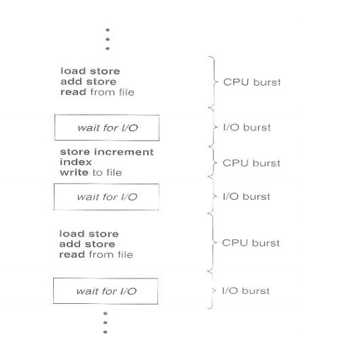
   Almost all processes alternate between two states in a continuing cycle, as shown in Figure below :

o  A CPU burst of performing calculations, and

o  An I/O burst, waiting for data transfer in or out of the system.

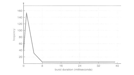
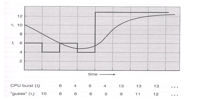
CPU bursts vary from process to process, and from program to program, but an extensive study shows frequency patterns similar to that shown in Figure

ü               CPU Scheduler

ü Whenever the CPU becomes idle, it is the job of the CPU Scheduler ( a.k.a. the short-term scheduler ) to select another process from the ready queue to run next.

ü The storage structure for the ready queue and the algorithm used to select the next process are not necessarily a FIFO queue. There are several alternatives to choose from, as well as numerous adjustable parameters for each algorithm.

Preemptive Scheduling

·        CPU scheduling decisions take place under one of four conditions:

1.     When a process switches from the running state to the waiting state, such as for an I/O request or invocation of the wait( ) system call.

2.     When a process switches from the running state to the ready state, for example in response to an interrupt.

3.     When a process switches from the waiting state to the ready state, say at completion of I/O or a return from wait( ).

4.     When a process terminates.

·        For conditions 1 and 4 there is no choice - A new process must be selected.

·        For conditions 2 and 3 there is a choice - To either continue running the current process, or select a different one.

·        If scheduling takes place only under conditions 1 and 4, the system is said to be non-preemptive, or cooperative. Under these conditions, once a process starts running it keeps running, until it either voluntarily blocks or until it finishes. Otherwise the system is said to be preemptive.

·        Windows used non-preemptive scheduling up to Windows 3.x, and started using pre-emptive scheduling with Win95. Macs used non-preemptive prior to OSX, and pre-emptive since then. Note that pre-emptive scheduling is only possible on hardware that supports a timer interrupt.

·        Note that pre-emptive scheduling can cause problems when two processes share data, because one process may get interrupted in the middle of updating shared data structures.

·        Preemption can also be a problem if the kernel is busy implementing a system call (e.g. updating critical kernel data structures) when the preemption occurs. Most modern UNIX deal with this problem by making the process wait until the system call has either completed or blocked before allowing the preemption Unfortunately this solution is problematic for real-time systems, as real-time response can no longer be guaranteed.

·        Some critical sections of code protect themselves from concurrency problems by disabling interrupts before entering the critical section and re-enabling interrupts on exiting the section. Needless to say, this should only be done in rare situations, and only on very short pieces of code that will finish quickly, (usually just a few machine instructions.)

Dispatcher

ü The dispatcher is the module that gives control of the CPU to the process selected by the scheduler. This function involves:

o  Switching context.

o  Switching to user mode.

o  Jumping to the proper location in the newly loaded program.

ü The dispatcher needs to be as fast as possible, as it is run on every context switch. The time consumed by the dispatcher is known as dispatch latency.

Scheduling Algorithms

ü The following subsections will explain several common scheduling strategies, looking at only a single CPU burst each for a small number of processes. Obviously real systems have to deal with a lot more simultaneous processes executing their CPU-I/O burst cycles.

First-Come First-Serve Scheduling, FCFS

ü        FCFS is very simple - Just a FIFO queue, like customers waiting in line at the bank or the post office or at a copying machine.

ü        Unfortunately, however, FCFS can yield some very long average wait times, particularly if the first process to get there takes a long time. For example, consider the following three processes:

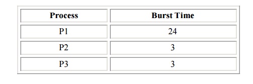
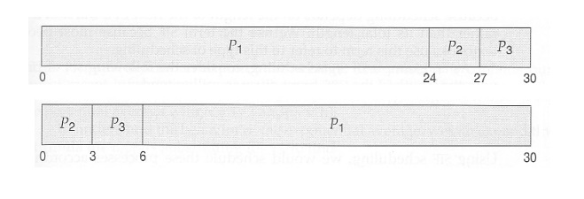
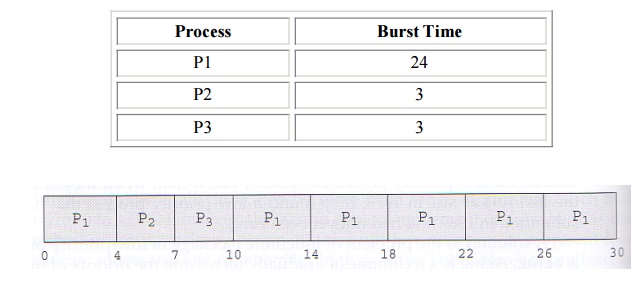
·        In the first Gantt chart below, process P1 arrives first. The average waiting time for the three processes is ( 0 + 24 + 27 ) / 3 = 17.0 ms.

·        In the second Gantt chart below, the same three processes have an average wait time of ( 0 + 3 + 6 ) / 3 = 3.0 ms. The total run time for the three bursts is the same, but in the second case two of the three finish much quicker, and the other process is only delayed by a short amount.

Shortest-Job-First Scheduling, SJF

The idea behind the SJF algorithm is to pick the quickest fastest little job that needs to be done, get it out of the way first, and then pick the next smallest fastest job to do next.

Technically this algorithm picks a process based on the next shortest CPU burst, not the overall process time.

For example, the Gantt chart below is based upon the following CPU burst times, ( and the assumption that all jobs arrive at the same time. )

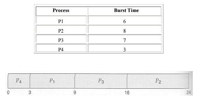
In the case above the average wait time is ( 0 + 3 + 9 + 16 ) / 4 = 7.0 ms, ( as opposed to 10.25 ms for FCFS for the same processes. )

SJF can be either preemptive or non-preemptive. Preemption occurs when a new process arrives in the ready queue that has a predicted burst time shorter than the time remaining in the process whose burst is currently on the CPU. Preemptive SJF is sometimes referred to as shortest remaining time first scheduling.

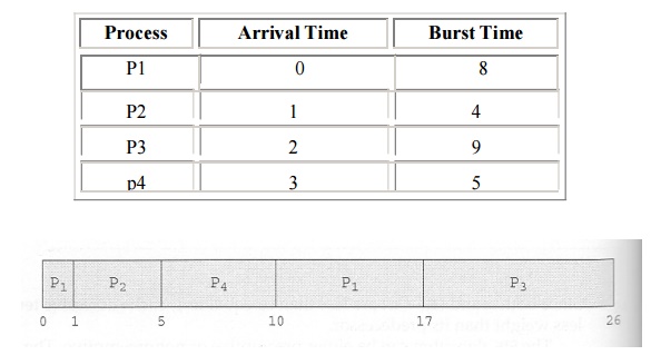
For example, the following Gantt chart is based upon the following data:

· The average wait time in this case is

((5 - 3 ) + ( 10 - 1 ) + ( 17 - 2 ) ) / 4 = 26 / 4 = 6.5 ms.

( As opposed to 7.75 ms for non-preemptive SJF or 8.75 for FCFS. )

Priority Scheduling

·        Priority scheduling is a more general case of SJF, in which each job is assigned a priority and the job with the highest priority gets scheduled first. (SJF uses the inverse of the next expected burst time as its priority - The smaller the expected burst, the higher the priority. )

·        Note that in practice, priorities are implemented using integers within a fixed range, but there is no agreed-upon convention as to whether "high" priorities use large numbers or small numbers.

·        For example, the following Gantt chart is based upon these process burst times and priorities, and yields an average waiting time of 8.2 ms:

·        Priorities can be assigned either internally or externally. Internal priorities are assigned by the OS using criteria such as average burst time, ratio of CPU to I/O activity, system resource use, and other factors available to the kernel. External priorities are assigned by users, based on the importance of the job, fees paid, politics, etc.

Round Robin Scheduling

·        Round robin scheduling is similar to FCFS scheduling, except that CPU bursts are assigned with limits called time quantum.

·        When a process is given the CPU, a timer is set for whatever value has been set for a time quantum.

o   If the process finishes its burst before the time quantum timer expires, then it is swapped out of the CPU just like the normal FCFS algorithm.

     If the timer goes off first, then the process is swapped out of the CPU and moved to the back end of the ready queue.

§     The ready queue is maintained as a circular queue, so when all processes have had a turn, then the scheduler gives the first process another turn, and so on.

§     RR scheduling can give the effect of all processors sharing the CPU equally, although the average wait time can be longer than with other scheduling algorithms. In the following example the average wait time is 5.66 ms.

·        The performance of RR is sensitive to the time quantum selected. If the quantum is large enough, then RR reduces to the FCFS algorithm; If it is very small, then each process gets 1/nth of the processor time and share the CPU equally.

·        BUT, a real system invokes overhead for every context switch, and the smaller the time quantum the more context switches there are. ( See Figure 5.4 below. ) Most modern systems use time quantum between 10 and 100 milliseconds, and context switch times on the order of 10 microseconds, so the overhead is small relative to the time quantum.

·        In general, turnaround time is minimized if most processes finish their next cpu burst within one time quantum. For example, with three processes of 10 ms bursts each, the average turnaround time for 1 ms quantum is 29, and for 10 ms quantum it reduces to 20.

·        However, if it is made too large, then RR just degenerates to FCFS. A rule of thumb is that 80% of CPU bursts should be smaller than the time quantum.

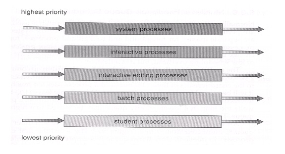
Multilevel Queue Scheduling

ü When processes can be readily categorized, then multiple separate queues can be established, each implementing whatever scheduling algorithm is most appropriate for that type of job, and/or with different parametric adjustments.

ü Scheduling must also be done between queues, that is scheduling one queue to get time relative to other queues. Two common options are strict priority ( no job in a lower priority queue runs until all higher priority queues are empty ) and round-robin ( each queue gets a time slice in turn, possibly of different sizes. )

ü Note that under this algorithm jobs cannot switch from queue to queue - Once they are assigned a queue, that is their queue until they finish

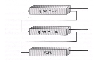
Multilevel Feedback-Queue Scheduling

1.3 Multilevel feedback queue scheduling is similar to the ordinary multilevel queue scheduling described above, except jobs may be moved from one queue to another for a variety of reasons:

o   If the characteristics of a job change between CPU-intensive and I/O intensive, then it may be appropriate to switch a job from one queue to another.

o   Aging can also be incorporated, so that a job that has waited for a long time can get bumped up into a higher priority queue for a while.

ü Some of the parameters which define one of these systems include:

o  The number of queues.

o  The scheduling algorithm for each queue.

o       The methods used to upgrade or demote processes from one queue to another. ( Which may be different. )

o  The method used to determine which queue a process enters initially.