Branch Prediction method

Branch Prediction method

1. Static Branch Prediction method

Static branch predictors      are   used              in       processors      where          the         expectation        is    that branch behavior is highly predictable at compile-time; static prediction can also be used to assist dynamic predictors.

An architectural feature that supports static branch predication, namely delayed branches. Delayed branches expose a pipeline hazard so that the compiler can reduce the penalty associated with the hazard. The effectiveness of this technique partly depends on whether we correctly guess which way a branch will go. Being able to accurately predict a branch at compile time is also helpful for scheduling data hazards. Loop unrolling is on branches. Loop unrolling is on simple example of this; another example arises from conditional selection branches.

Consider the following code segment:

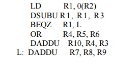
LD     R1, 0(R2)

DSUBU R 1 , R 1 , R 3

BEQZ         R1, L

OR    R4, R5, R6

DADDU     R10, R4, R3

L:  DADDU          R7, R8, R9

The dependence of the DSUBU and BEQZ on the LD instruction means that a stall will be needed after the LD. Suppose this branch was almost always taken and that the value of R7 was not needed on the fall-through path. Then we could increase the speed of the program by moving the instruction DADD R7,R8,R9 to the position after the LD. If the branch was rarely taken and that the value of R4 was not needed on the taken path, then we could contemplate moving the OR instruction after the LD.

To perform these optimizations, we need to predict the branch statically when we compile the program. There are several different methods to statically predict branch behavior. The simplest scheme is to predict a branch as taken. This scheme has an average misprediction rate that is equal to the untaken branch frequency, which for the SPEC programs is 34%.

Unfortunately, the misprediction rate ranges from not very accurate (59%) to highly accurate (9%).

A better alternative is to predict on the basis of branch direction, choosing backward-going branches to be taken and forward-going branches to be not taken. For some programs and compilation systems, the frequency of forward taken branches may be significantly less than 50%, and this scheme will do better than just predicting all branches as taken. In the SPEC programs, however, more than half of the forward-going branches are taken. Hence, predicting all branches as taken is the better approach.

A still more accurate technique is to predict branches on the basis of profile information collected from earlier runs. The key observation that makes this worthwhile is that the behavior of branches is often bimodally distributed; that is, an individual branch is often highly biased toward taken or untaken.

2. Reduce Branch Costs with Dynamic Hardware Prediction

2.1.         Basic Branch Prediction and Branch-Prediction Buffers

Ø The simplest dynamic branch-prediction scheme is a branch-pr ediction buffer or branch history table.

Ø A branch-prediction buffer is a small memory indexed by the lower portion of the address of the branch instruction.

Ø The memory contains a bit that says whether the branch was recently taken or not. if the prediction is correct—it may have been put there by another branch that has the same low-order address bits.

Ø The prediction is a hint that is assumed to be correct, and fetching begins in the predicted direction. If the hint turns out to be wrong, the prediction bit is inverted and stored back.

Ø The performance of the buffer depends on both how often the prediction is for the branch of interest and how accurate the prediction is when it matches.

Ø This simple one-bit prediction scheme has a performance shortcoming: Even if a branch is almost always taken, we will likely predict incorrectly twice, rather than once, when it is not taken.

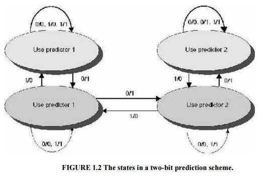
The two bits are used to encode the four states in the system. In a counter implementation, the counters are incremented when a branch is taken and decremented when it is not taken; the counters saturate at 00 or 11.

One complication of the two-bit scheme is that it updates the prediction bits more often than a one-bit predictor, which only updates the prediction bit on a mispredict. Since we typically read the prediction bits on every cycle, a two-bit predictor will typically need both a read and a write access port.

The two-bit scheme is actually a specialization of a more general scheme that has an n-bit saturating counter for each entry in the prediction buffer. With an n-bit counter, the counter can take on values between 0 and 2 ⁿ – 1: when the counter is greater than or equal to one half of its maximum value (2 ^n-1), the branch is predicted as taken; otherwise, it is predicted untaken.

To exploit more ILP, the accuracy of our branch prediction becomes critical, this problem in two ways: by increasing the size of the buffer and by increasing the accuracy of the scheme we use for each prediction.

2.2. Correlating Branch Predictors:

These two-bit predictor schemes use only the recent behavior of a single branch to predict the future behavior of that branch. It may be possible to improve the prediction accuracy if we also look at the recent behavior of other branches rather than just the branch we are trying to predict.

Consider a small code fragment from the SPEC92 benchmark

if (aa==2) aa=0;

if (bb==2) bb=0;

if (aa!=bb) {

Here is the MIPS code that we would typically generate for this code fragment assuming that aa and bb are assigned to registers R1 and R2:

          DSUBUI     R3, R1, #2

          BNEZ         R3, L1; branch b1 (aa! =2)

          DADD        R1, R0, R0; aa=0

L1:    DSUBUI     R3, R2, #2

          BNEZ         R3, L2; branch b2 (bb! =2)

          DADD        R2, R0, R0; bb=0

L2:    DSUBU      R3, R1, R2; R3=aa-bb

          BEQZ         R3, L3; branch b3 (aa==bb)

Let’s label these branches b1, b2, and b3. The key observation is that the behavior of branch b3 is correlated with the behavior of branches b1 and b2. Clearly, if branches b1 and b2 are both not taken (i.e., the if conditions both evaluate to true and aa and bb are both assigned 0), then b3 will be taken, since aa and bb are clearly equal. A predictor that uses only the behavior of a single branch to predict the outcome of that branch can never capture this behavior.

Branch predictors that use the behavior of other branches to make a prediction are called correlating predictors or two-level predictors.

2.3. Tournament Predictors: Adaptively Combining Local and Global Predictors

The primary motivation for correlating branch predictors came from the observation that the standard 2-bit predictor using only local information failed on some important branches and that by adding global information, the performance could be improved. Tournament predictors take this insight to the next level, by using multiple predictors, usually one based on global information and one based on local information, and combining them with a selector. Tournament predictors can achieve both better accuracy at medium sizes (8Kb-32Kb) and also make use of very large numbers of prediction bits effectively.

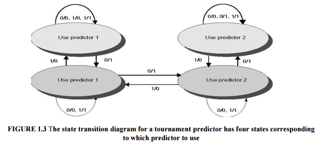
Tournament predictors are the most popular form of multilevel branch predictors. A multilevel branch predictor use several levels of branch prediction tables together with an algorithm for choosing among the multiple predictors; Existing tournament predictors use a 2-bit saturating counter per branch to choose among two different predictors. The four states of the counter dictate whether to use predictor 1 or predictor 2. The state transition diagram is shown in Figure 1.3

2.4. High Performance Instruction Delivery

Branch Target Buffers

A branch-prediction cache that stores the predicted address for the next instruction after a branch is called a branch-target buffer or branch-target cache.

For the classic, five-stage pipeline, a branch-prediction buffer is accessed during the ID cycle, so that at the end of ID we know the branch-target address (since it is computed during ID), the fall-through address (computed during IF), and the prediction. Thus, by the end of ID we know enough to fetch the next predicted instruction. For a branch-target buffer, we access the buffer during the IF stage using the instruction address of the fetched instruction, a possible branch, to index the buffer. If we get a hit, then we know the predicted instruction address at the end of the IF cycle, which is one cycle earlier than for a branch-prediction buffer.

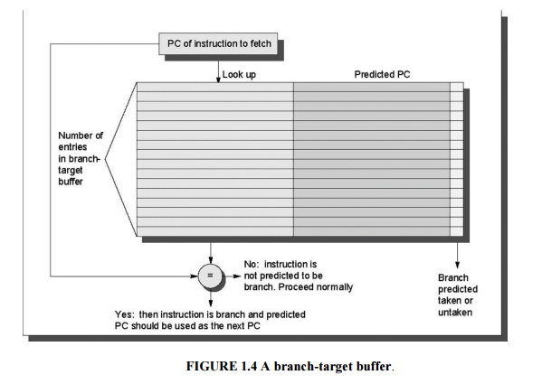
Because we are predicting the next instruction address and will send it out before decoding the instruction, we must know whether the fetched instruction is predicted as a taken branch. Figure 1.4 shows what the branch-target buffer looks like. If the PC of the fetched instruction matches a PC in the buffer, then the corresponding predicted PC is used as the next PC.

If a matching entry is found in the branch-target buffer, fetching begins immediately at the predicted PC. Note that the entry must be for this instruction, because the predicted PC will be sent out before it is known whether this instruction is even a branch. If we did not check whether the entry matched this PC, then the wrong PC would be sent out for instructions that were not branches, resulting in a slower processor. We only need to store the predicted-taken branches in the branch-target buffer, since an untaken branch follows the same strategy as a non branch.

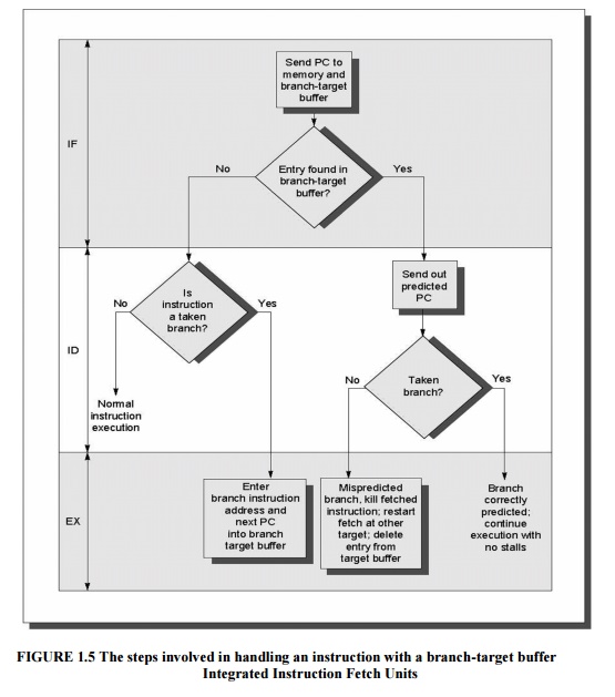
Figure 1.5 shows the steps followed when using a branch-target buffer and where these steps occur in the pipeline. From this we can see that there will be no branch delay if a branch-prediction entry is found in the buffer and is correct.

The recent designs have used an integrated instruction fetch unit that integrates several functions:

1.  Integrated branch prediction: the branch predictor becomes part of the instruction fetch unit and is constantly predicting branches, so to drive the fetch pipeline.

2.  Instruction prefetch: to deliver multiple instructions per clock, the instruction fetch unit will likely need to fetch ahead. The unit autonomously manages the prefetching of instructions, integrating it with branch prediction.

3.  Instruction memory access and buffering:.The instruction fetch unit also provides buffering, essentially acting as an on-demand unit to provide instructions to the issue stage as needed and in the quantity needed

Return Address Predictors:

The concept of a small buffer of return addresses operating as a stack is used to predict the return address. This structure caches the most recent return addresses: pushing a return address on the stack at a call and popping one off at a return. If the cache is sufficiently large, it will predict the returns perfectly.