Two Way ANOVA

TWO-WAY ANOVA

In two-way ANOVA a study variable is compared over three or more groups, controlling for another variable. The grouping is taken as one factor and the control is taken as another factor. The grouping factor is usually known as Treatment. The control factor is usually called Block. The accuracy of the test in two -way ANOVA is considerably higher than that of the one-way ANOVA, as the additional factor, block is used to reduce the error variance.

In two-way ANOVA, the data can be represented in the following tabular form.

Blocks

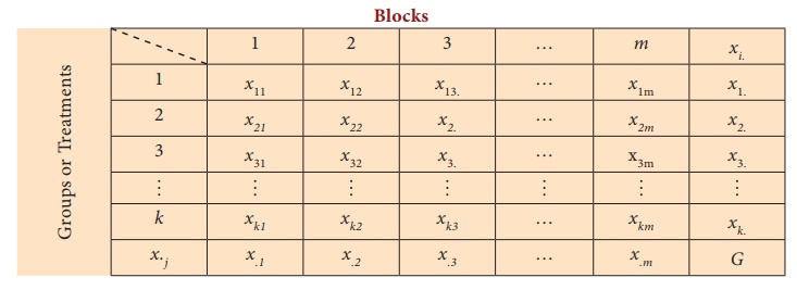
We use the following notations.

x_ij - i^th treatment value from the j^th block, i = 1,2, ..., k; j = 1,2, ..., m.

The i^th treatment total - x_i =  , i 1, 2, ..., k

The j^th block total - x _{. j} x_ij , j 1, 2, ..., m

Note that, k × m = n, where m = number of blocks, and k = number of treatments (groups) and n is the total number of observations in the study.

The total variation present in the observations x_ij can be split into the following three components:

(i) The variation between treatments (groups)

(ii) The variation between blocks.

(ii) The variation inherent within a particular setting or combination of treatment and block.

1. Test Procedure

Steps involved in two-way ANOVA are:

Step 1 : In two-way ANOVA we have two pairs of hypotheses, one for treatments and one for the blocks.

Framing Hypotheses

Null Hypotheses

H₀₁: There is no significant difference among the population means of different groups (Treatments)

H₀₂: There is no significant difference among the population means of different Blocks

Alternative Hypotheses

H₁₁: Atleast one pair of treatment means differs significantly

H₁₂: Atleast one pair of block means differs significantly

Step 2 : Data is presented in a rectangular table form as described in the previous section.

Step 3 : Level of significance α.

Step 4 : Test Statistic

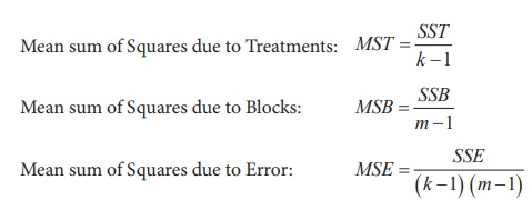
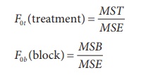
F_0t (treatments) = MST / MSE

F_0b (block) = MSB / MSE

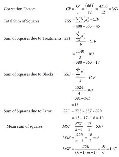
To find the test statistic we have to find the following intermediate values.

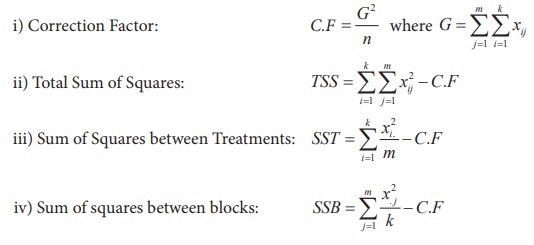
v) Sum of Squares due to Error: SSE = TSS-SST-SSB

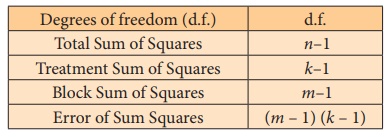
vi) Degrees of freedom

vii) Mean Sum of Squares

Step 5 : Calculation of the Test Statistic

ANOVA Table (two-way)

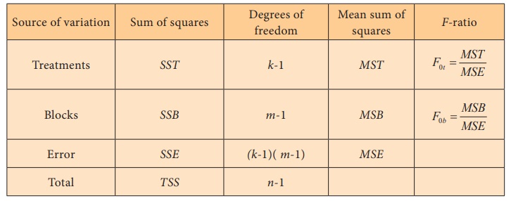
Step 6 : Critical values

Critical value for treatments = f_{(k-1,(m-1)(k-1)),α}

Critical value for blocks = f_{(m-1, (m-1)(k-1)),α}

Step 7 : Decision

For Treatments: If the calculated F_0t value is greater than the corresponding critical value, then we reject the null hypothesis and conclude that there is significant difference among the treatment means, in atleast one pair.

For Blocks: If the calculated F_0b value is greater than the corresponding critical value, then we reject the null hypothesis and conclude that there is significant difference among the block means, in at least one pair.

2. Merits and Demerits of two-way ANOVA

Merits

·              Any number of blocks and treatments can be used.

·              Number of units in each block should be equal.

·              It is the most used design in view of the smaller total sample size since we are studying two variable at a time.

Demerits

·              If the number of treatments is large enough, then it becomes difficult to maintain the homogeneity of the blocks.

·              If there is a missing value, it cannot be ignored. It has to be replaced with some function of the existing values and certain adjustments have to be made in the analysis. This makes the analysis slightly complex.

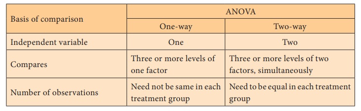
Comparison between one-way ANOVA and two-way ANOVA

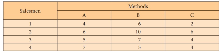
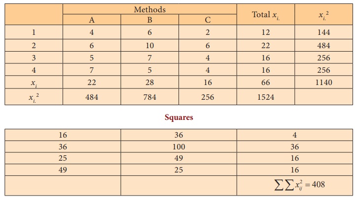
Example 3.6

A reputed marketing agency in India has three different training programs for its salesmen. The three programs are Method – A, B, C. To assess the success of the programs, 4 salesmen from each of the programs were sent to the field. Their performances in terms of sales are given in the following table.

Test whether there is significant difference among methods and among salesmen.

Solution:

Step 1 : Hypotheses

Null Hypotheses: H₀₁ : μ_M1= μ_M2 = μ_M3 (for treatments)

That is, there is no significant difference among the three programs in their mean sales.

H₀₂ : μ_S1 = μ_S2 = μ_S3 = μ_S4 (for blocks)

Alternative Hypotheses:

H₁₁ : At least one average is different from the other, among the three programs.

H₁₂ : At least one average is different from the other, among the four salesmen.

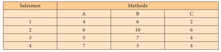
Step 2 : Data

Step 3 : Level of significance α = 5%

Step 4 : Test Statistic

Step-5 : Calculation of the Test Statistic

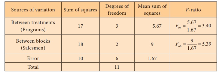
ANOVA Table (two-way)

Step 6 : Critical values

f_{(3, 6),0.05} = 4.7571 (for treatments)

f_{(2, 6),0.05} = 5.1456 (for blocks)

Step 7 : Decision

(i) Calculated F_0t = 3.40 < f_{(3, 6),0.05} = 4.7571, the null hypothesis is not rejected and we conclude that there is significant difference in the mean sales among the three programs.

(ii) Calculate F_0b = 5.39 > f_{(2, 6),0.05} = 5.1456, the null hypothesis is rejected and conclude that there does not exist significant difference in the mean sales among the four salesmen.

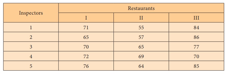
Example 3.7

The illness caused by a virus in a city concerning some restaurant inspectors is not consistent with their evaluations of cleanliness of restaurants. In order to investigate this possibility, the director has five restaurant inspectors to grade the cleanliness of three restaurants. The results are shown below.

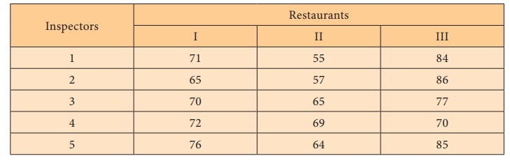
Carry out two-way ANOVA at 5% level of significance.

Solution:

Step 1 :

Null hypotheses

H_0I : µ₁ = µ ₂ = µ ₃ = µ ₄ = µ₅ (For inspectors - Treatments)

That is, there is no significant difference among the five inspectors over their mean cleanliness scores

H_0R : μ_I = μ_II = μ_III (For restaurants - Blocks)

That is, there is no significant difference among the three restaurants over their mean cleanliness scores

Alternative Hypotheses

H_1I: At least one mean is different from the other among the Inspectors

H_1R: At least one mean is different from the other among the Restaurants.

Step 2 : Data

Step 3 : Level of significance α = 5%

Step 4 : Test Statistic

For inspectors: F_0a (treatments) = = MST / MSE

For restaurants: F_0b (blocks) = MSE / MSB

Step-5 : Calculation of the Test Statistic

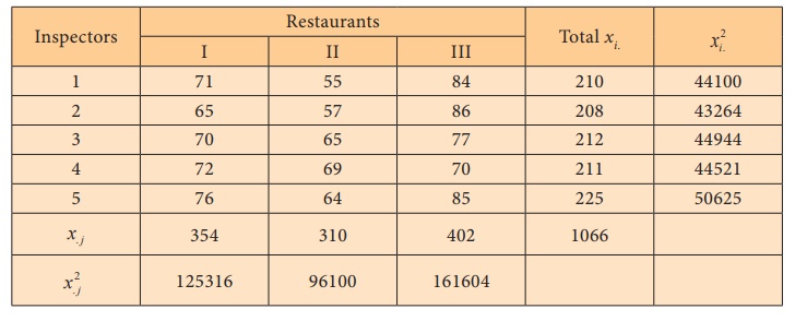
Squares

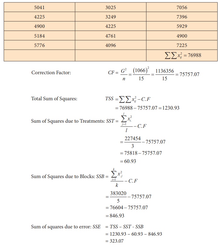
ANOVA Table (two-way)

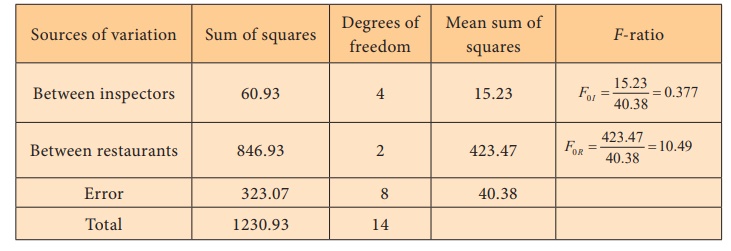
Step 6 : Critical values

f_{(4, 8),0.05} = 3.838 (for inspectors)

f_{(2, 8),0.05} = 4.459 (for restaurants)

Step 7 : Decision

(i) As F_0I = 0.377 < f_{(4, 8),0.05} = 3.838, the null hypothesis is not rejected and we conclude that there is no significant difference among the mean cleanliness scores of inspectors.

(ii) As F_0R = 10.49 > f_{(2, 8),0.05} = 4.459, the null hypothesis is rejected and we conclude that there exists significant difference in atleast one pair of restaurants over their mean cleanliness scores.