One-way ANOVA

ANALYSIS OF VARIANCE (ANOVA)

In chapter 2, testing equality means of two normal populations based on independent small samples was discussed. When the number of populations is more than 2, those methods cannot be applied.

ANOVA is used when we want to test the equality of means of more than two populations. For example, through ANOVA, one may compare the average yield of several varieties of a crop or average mileages of different brands of cars.

ANOVA cannot be used in all situations and for all types of variables. It is based on certain assumptions, and they are listed below:

1. The observations follow normal distribution.

2. The samples are independent.

3. The population variances are equal and unknown.

According to R.A. Fisher ANOVA is the “Separation of variance, ascribable to one group of causes from the variance ascribable to other groups”.

The data may be classified with respect to different levels of a single factor/or different levels of two factors.

The former is called one-way classified data and the latter is called two-way classified data.

Applications of ANOVA technique to these kinds of data are discussed in the following sections.

One-way ANOVA

ANOVA is a statistical technique used to determine whether differences exist among three or more population means.

In one-way ANOVA the effect of one factor on the mean is tested. It is based on independent random samples drawn from k – different levels of a factor, also called treatments.

The following notations are used in one-way ANOVA. The data can be represented in the following tabular structure.

Data representation for one-way ANOVA

x_ij - the j ^th sample value from the ith treatment, j = 1, 2, …,n_i, i =1, 2,…,k

k - number of treatments compared.

x_i. - the sample total of i^th treatment.

n_i - the number of observations in the i^th treatment.

The total variation in the observations x_ij can be split into the following two components

(i) variation between the levels or the variation due to different bases of classification, commonly known as treatments.

(ii) The variation within the treatments i.e. inherent variation among the observations within levels.

Causes involved in the first type of variation are known as assignable causes. The causes leading to the second type of variation are known as chance or random causes.

The first type of variation that is due to assignable causes, can be detected and controlled by human endeavor and the second type of variation that is due to chance causes, is beyond the human control.

Test Procedure

Let the observations x_ij, j = 1, 2, …, n_i for treatment i, be assumed to come from N(μ_i, σ²) population, i = 1, 2, …, k where σ² is unknown.

Step 1 : Framing Hypotheses

Null Hypothesis H₀ : μ₁ = μ₂ = ... = μ_k

That is, there is no significant difference among the population means of k treatments.

Alternative Hypothesis

H₁: μ_i≠μ_j for atleast one pair (i,j); i, j =1,2,...,k; i ≠ j

That is, at least one pair of means differ significantly.

Step 2 : Data

Data is presented in the tabular form as described in the previous section

Step 3 : Level of significance : α

Step 4 : Test Statistic

F = MST/MSE which follows F_{(k-1, n-k)}, under H₀

To evaluate the test statistic we compute the following:

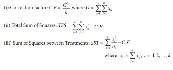
(iv) Sum of Squares due to Error: SSE = TSS – SST

Degrees of Freedom (d.f)

Mean Sum of Squares

Mean Sum of Squares due to treatment: MST = SST / k −1

Mean Sum of Squares due to Error: MSE = SSE / n – k

Step 5 : Calculation of Test statistic

ANOVA Table (one-way)

Step 6 : Critical value

f_e = f_{(k-1, n-k),α.}

Step 7 : Decision

If F₀ < f_{(k-1, n-k),α} then reject H₀.

Merits and Demerits of One-Way ANOVA

Merits

·              Layout is very simple and easy to understand.

·              Gives maximum degrees of freedom for error.

Demerits

·              Population variances of experimental units for different treatments need to be equal.

·              Verification of normality assumption may be difficult.

Example 3.4

Three different techniques namely medication, exercises and special diet are randomly assigned to (individuals diagnosed with high blood pressure) lower the blood pressure. After four weeks the reduction in each person’s blood pressure is recorded. Test at 5% level, whether there is significant difference in mean reduction of blood pressure among the three techniques.

Solution:

Step 1 : Hypotheses

Null Hypothesis: H₀: µ₁ = µ₂ = µ₃

That is, there is no significant difference among the three groups on the average reduction in blood pressure.

Alternative Hypothesis: H₁: μ_i ≠ μ_j for atleast one pair (i, j); i, j = 1, 2, 3; i ≠ j.

That is, there is significant difference in the average reduction in blood pressure in atleast one pair of treatments.

Step 2 : Data

Step 3 : Level of significance α = 0.05

Step 4 : Test statistic

F₀ = MST / MSE

Step 5 : Calculation of Test statistic

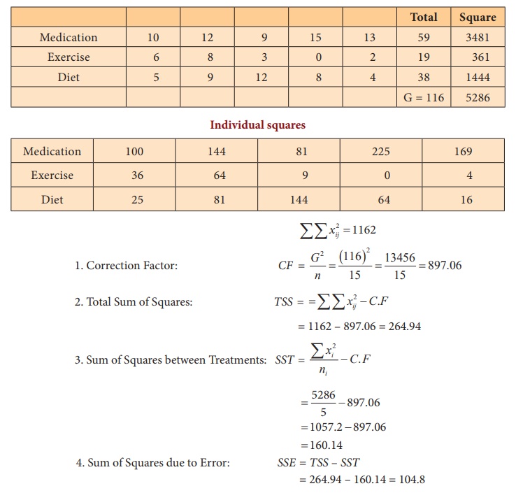
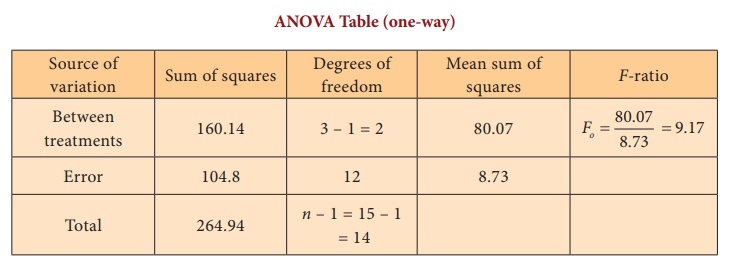
Step 6 : Critical value

f_{(2, 12),0.05} = 3.8853.

Step 7 : Decision

As F₀ = 9.17 > f_{(2, 12),0.05} = 3.8853, the null hypothesis is rejected. Hence, we conclude that there exists significant difference in the reduction of the average blood pressure in atleast one pair of techniques.

Example 3.5

Three composition instructors recorded the number of spelling errors which their students made on a research paper. At 1% level of significance test whether there is significant difference in the average number of errors in the three classes of students.

Solution:

Step 1 : Hypotheses

Null Hypothesis: H₀ : µ₁ = µ₂ = µ₃

That is there is no significant difference among the mean number of errors in the three classes of students.

Alternative Hypothesis

H₁ : μ_i ≠ μ_j for at one pair (i, j); i,j = 1,2,3; i ≠ j.

That is, atleast one pair of groups differ significantly on the mean number of errors.

Step 2 : Data

Step 3 : Level of significance α = 5%

Step 4 : Test Statistic

F₀ = MST / MSE

Step 5 : Calculation of Test statistic

Individual squares

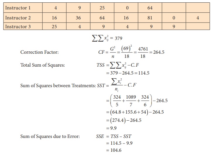
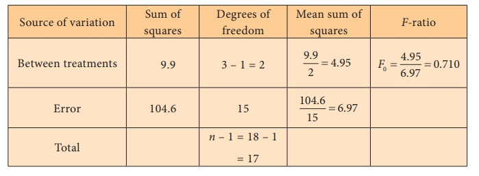
ANOVA Table

Step 6 : Critical value

The critical value = f_{(15, 2),0.05} = 3.6823.

Step 7 : Decision

As F₀ = 0.710 < f_{(15, 2),0.05} = 3.6823, null hypothesis is not rejected. There is no enough evidence to reject the null hypothesis and hence we conclude that the mean number of errors made by these three classes of students are not equal.