Statistical Analysis of Data

Statistical Analysis of Data

In the previous section we noted that the result of an analysis is best expressed as a confidence interval. For example, a 95% confidence interval for the mean of five re- sults gives the range in which we expect to find the mean for 95% of all samples of equal size, drawn from the same population. Alternatively, and in the absence of de- terminate errors, the 95% confidence interval indicates the range of values in which we expect to find the population’s true mean.

The probabilistic nature of a confidence interval provides an opportunity to ask and answer questions comparing a sample’s mean or variance to either the accepted values for its population or similar values obtained for other samples. For example, confidence intervals can be used to answer questions such as “Does a newly devel- oped method for the analysis of cholesterol in blood give results that are signifi- cantly different from those obtained when using a standard method?” or “Is there a significant variation in the chemical composition of rainwater collected at different sites downwind from a coalburning utility plant?” In this section we introduce a general approach to the statistical analysis of data.

Significance Testing

Let’s consider the following problem. Two sets of blood samples have been collected from a patient receiving medication to lower her concentration of blood glucose. One set of samples was drawn immediately before the medication was adminis- tered; the second set was taken several hours later. The samples are analyzed and their respective means and variances reported. How do we decide if the medication was successful in lowering the patient’s concentration of blood glucose?

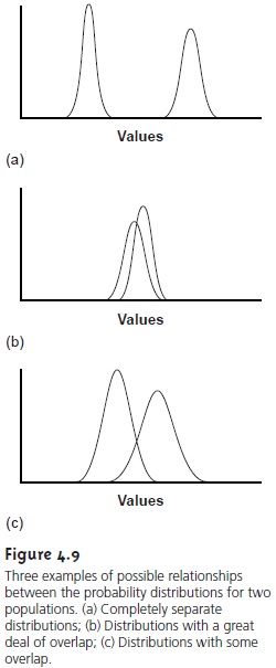
One way to answer this question is to construct probability distribution curves for each sample and to compare the curves with each other. Three possible out- comes are shown in Figure 4.9. In Figure 4.9a, the probability distribution curves are completely separated, strongly suggesting that the samples are significantly dif- ferent. In Figure 4.9b, the probability distributions for the two samples are highly overlapped, suggesting that any difference between the samples is insignificant. Figure 4.9c, however, presents a dilemma. Although the means for the two samples ap- pear to be different, the probability distributions overlap to an extent that a signifi- cant number of possible outcomes could belong to either distribution. In this case we can, at best, only make a statement about the probability that the samples are significantly different.

The process by which we determine the probability that there is a significant difference between two samples is called significance testing or hypothesis testing. Before turning to a discussion of specific examples, however, we will first establish a general approach to conducting and interpreting significance tests.

Constructing a Significance Test

A significance test is designed to determine whether the difference between two or more values is too large to be explained by indeterminate error. The first step in constructing a significance test is to state the experimental problem as a yes- or-no question, two examples of which were given at the beginning of this sec- tion. A null hypothesis and an alternative hypothesis provide answers to the ques- tion. The null hypothesis, H₀, is that indeterminate error is sufficient to explain any difference in the values being compared. The alternative hypothesis, H_A, is that the difference between the values is too great to be explained by random error and, therefore, must be real. A significance test is conducted on the null hy- pothesis, which is either retained or rejected. If the null hypothesis is rejected, then the alternative hypothesis must be accepted. When a null hypothesis is not rejected, it is said to be retained rather than accepted. A null hypothesis is re- tained whenever the evidence is insufficient to prove it is incorrect. Because of the way in which significance tests are conducted, it is impossible to prove that a null hypothesis is true.

The difference between retaining a null hypothesis and proving the null hy- pothesis is important. To appreciate this point, let us return to our example on de- termining the mass of a penny. After looking at the data in Table 4.12, you might pose the following null and alternative hypotheses

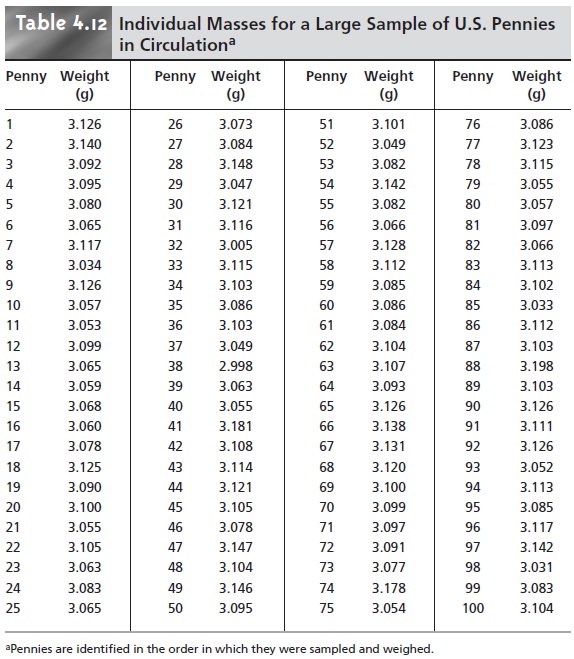
·              H₀: Any U.S. penny in circulation has a mass that falls in the range of 2.900–3.200 g

·              H_A: Some U.S. pennies in circulation have masses that are less than 2.900 g or more than 3.200 g.

To test the null hypothesis, you reach into your pocket, retrieve a penny, and deter- mine its mass. If the mass of this penny is 2.512 g, then you have proved that the null hypothesis is incorrect. Finding that the mass of your penny is 3.162 g, how- ever, does not prove that the null hypothesis is correct because the mass of the next penny you sample might fall outside the limits set by the null hypothesis.

After stating the null and alternative hypotheses, a significance level for the analysis is chosen. The significance level is the confidence level for retaining the null hypothesis or, in other words, the probability that the null hypothesis will be incor- rectly rejected. In the former case the significance level is given as a percentage (e.g., 95%), whereas in the latter case, it is given as α, where α is defined as

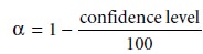
Thus, for a 95% confidence level, α is 0.05.

Next, an equation for a test statistic is written, and the test statistic’s critical value is found from an appropriate table. This critical value defines the breakpoint between values of the test statistic for which the null hypothesis will be retained or rejected. The test statistic is calculated from the data, compared with the critical value, and the null hypothesis is either rejected or retained. Finally, the result of the significance test is used to answer the original question.

One-Tailed and Two-Tailed Significance Tests

Consider the situation when the accuracy of a new analytical method is evaluated by analyzing a standard reference material with a known μ. A sample of the standard is analyzed, and the sample’s mean is determined. The null hypothesis is that the sample’s mean is equal to μ

If the significance test is conducted at the 95% confidence level (α = 0.05), then the null hypothesis will be retained if a 95% confidence interval around X– contains μ. If the alternative hypothesis is

then the null hypothesis will be rejected, and the alternative hypothesis accepted if μ lies in either of the shaded areas at the tails of the sample’s probability distribution (Figure 4.10a). Each of the shaded areas accounts for 2.5% of the area under the probability distribution curve. This is called a two-tailed significance test because the null hypothesis is rejected for values of μ at either extreme of the sample’s prob- ability distribution.

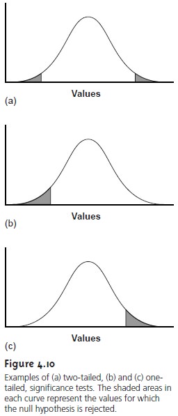
The alternative hypothesis also can be stated in one of two additional ways

for which the null hypothesis is rejected if μ falls within the shaded areas shown in Figure 4.10(b) and Figure 4.10(c), respectively. In each case the shaded area repre- sents 5% of the area under the probability distribution curve. These are examples of  one-tailed significance tests.

For a fixed confidence level, a two-tailed test is always the more conservative test because it requires a larger difference between X– and μ to reject the null hypothesis. Most significance tests are applied when there is no a priori expectation about the relative magnitudes of the parameters being compared. A two-tailed significance test, therefore, is usually the appropriate choice. One-tailed significance tests are reserved for situations when we have reason to expect one parameter to be larger or smaller than the other. For example, a one-tailed significance test would be appropriate for our earlier example regarding a medication’s effect on blood glucose levels since we believe that the medication will lower the concentration of glucose.

Errors in Significance Testing

Since significance tests are based on probabilities, their interpretation is naturally subject to error. As we have already seen, significance tests are carried out at a sig- nificance level, α, that defines the probability of rejecting a null hypothesis that is true. For example, when a significance test is conducted at α = 0.05, there is a 5% probability that the null hypothesis will be incorrectly rejected. This is known as a type 1 error, and its risk is always equivalent to α. Type 1 errors in two-tailed and one-tailed significance tests are represented by the shaded areas under the probabil- ity distribution curves in Figure 4.10.

The second type of error occurs when the null hypothesis is retained even though it is false and should be rejected. This is known as a type 2 error, and its probability of occurrence is β. Unfortunately, in most cases β cannot be easily calculated or estimated.

The probability of a type 1 error is inversely related to the probability of a type 2 error. Minimizing a type 1 error by decreasing α, for example, increases the likeli- hood of a type 2 error. The value of α chosen for a particular significance test, therefore, represents a compromise between these two types of error. Most of the examples in this text use a 95% confidence level, or α = 0.05, since this is the most frequently used confidence level for the majority of analytical work. It is not unusual, however, for more stringent (e.g. α = 0.01) or for more lenient (e.g. α = 0.10) confidence levels to be used.