Chapter: An Introduction to Parallel Programming : Parallel Hardware and Parallel Software
Parallel Program Design with example
PARALLEL PROGRAM DESIGN
So we’ve
got a serial program. How do we parallelize it? We know that in general we need
to divide the work among the processes/threads so that each process gets roughly
the same amount of work and communication is minimized. In most cases, we also
need to arrange for the processes/threads to synchronize and communicate.
Unfortunately,
there isn’t some mechanical process we can follow; if there were, we could
write a program that would convert any serial program into a parallel program,
but, as we noted in Chapter 1, in spite of a tremendous amount of work and some
progress, this seems to be a problem that has no universal solution.
However,
Ian Foster provides an outline of steps in his online book Designing and Building Parallel
Programs [19]:
Partitioning. Divide the computation to be performed and
the data operated on by the computation into small tasks. The focus
here should be on identifying tasks that can be executed in parallel.
Communication. Determine what communication needs to be
carried out among the tasks identified in the previous step.
Agglomeration or aggregation. Combine tasks and
communications identified in the first step into larger tasks. For example,
if task A must be executed before task B can be executed, it may make sense to
aggregate them into a single composite task.
Mapping. Assign the composite tasks identified in the
previous step to processes/ threads. This should be done so that communication
is minimized, and each process/thread gets roughly the same amount of work.
This is
sometimes called Foster’s methodology.
An example
Let’s
look at a small example. Suppose we have a program that generates large
quan-tities of floating point data that it stores in an array. In order to get
some feel for the distribution of the data, we can make a histogram of the
data. Recall that to make a histogram, we simply divide the range of the data
up into equal sized subinter-vals, or bins, determine the number of
measurements in each bin, and plot a bar graph showing the relative sizes of
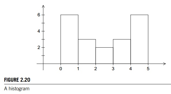
the bins. As a very small example, suppose our data are
1.3, 2.9, 0.4, 0.3, 1.3, 4.4, 1.7, 0.4, 3.2, 0.3, 4.9, 2.4, 3.1,
4.4, 3.9, 0.4, 4.2, 4.5, 4.9, 0.9.
Then the
data lie in the range 0–5, and if we choose to have five bins, the histogram
might look something like Figure 2.20.
A serial program
It’s
pretty straightforward to write a serial program that generates a histogram. We
need to decide what the bins are, determine the number of measurements in each
bin, and print the bars of the histogram. Since we’re not focusing on I/O,
we’ll limit ourselves to just the first two steps, so the input will be
the number of measurements, data count;
an array of data
count floats,
data;
the minimum value for the bin containing the smallest values, min meas;
the maximum value for the bin containing the largest values, max meas;
the number of bins, bin count;
The
output will be an array containing the number of elements of data that lie in
each bin. To make things precise, we’ll make use of the following data
structures:
bin
maxes. An array of bin_count floats
bin
counts. An array of bin_count ints
The
array bin
maxes will
store the upper bound for each bin, and bin counts will store the number of data elements in each
bin. To be explicit, we can define
bin_width
= (max_meas – min_meas)/bin_count
Then bin
maxes will be initialized by
for (b =
0; b < bin count; b++)
bin_maxes[b]
= min_meas + bin_width (b+1);
We’ll
adopt the convention that bin b will be all the measurements in the range
bin_maxes[b-1]
<= measurement < bin_maxes[b]
Of
course, this doesn’t make sense if b D 0, and in this case we’ll use the rule
that bin 0 will be the measurements in the range
min_meas
<= measurement < bin maxes[0]
This
means we always need to treat bin 0 as a special case, but this isn’t too
onerous. Once we’ve initialized bin maxes and assigned 0 to all the elements of
bin
counts, we can get the counts by using the following pseudo-code:
for (i =
0; i < data count; i++) {
bin =
Find_bin(data[i], bin_maxes, bin_count, min_meas);
bin_counts[bin]++;
}
The Find bin function returns the bin that data[i] belongs to. This could be a simple linear
search function: search through bin maxes until you find a bin b that satisfies
bin_maxes[b 1] <= data[i] < bin_maxes[b]
(Here
we’re thinking of bin
maxes[ 1] as min meas.) This will be fine if there aren’t very many
bins, but if there are a lot of bins, binary search will be much better.
Parallelizing the serial program
If we
assume that data
count is much
larger than bin
count, then
even if we use binary search in the Find bin function, the vast majority of the work in
this code will be in the loop that determines the values in bin counts. The focus of our paralleliza-tion should
therefore be on this loop, and we’ll apply Foster’s methodology to it. The
first thing to note is that the outcomes of the steps in Foster’s methodology
are by no means uniquely determined, so you shouldn’t be surprised if at any
stage you come up with something different.
For the
first step we might identify two types of tasks: finding the bin to which an
element of data belongs and incrementing the
appropriate entry in bin
counts.
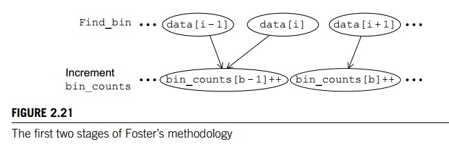
For the
second step, there must be a communication between the computation of the
appropriate bin and incrementing an element of bin counts. If we represent our tasks with ovals and
communications with arrows, we’ll get a diagram that looks something like that
shown in Figure 2.21. Here, the task labelled with “data[i]” is determining which bin the value data[i] belongs to, and the task labelled with “bin counts[b]++” is incrementing bin counts[b].
For any
fixed element of data, the tasks “find the bin b for element of data” and “increment bin counts[b]” can be aggregated, since the second can only
happen once the first has been completed.
However,
when we proceed to the final or mapping step, we see that if two pro-cesses or
threads are assigned elements of data that belong to the same bin b, they’ll both result in execution of the
statement bin
counts[b]++. If bin counts[b] is shared (e.g., the array bin counts is stored in shared-memory), then this will
result in a race condition. If bin
counts has been partitioned among the processes/threads, then updates to
its elements will require communication. An alternative is to store multiple
“local” copies of bin
counts and add the values in the local copies after all the calls to Find bin.
If the
number of bins, bin count, isn’t absolutely gigantic,
there shouldn’t be a problem with this. So let’s pursue this alternative, since
it is suitable for use on both shared- and distributed-memory systems.
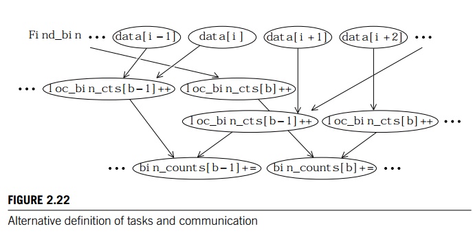
In this
setting, we need to update our diagram so that the second collection of tasks
increments loc bin
cts[b]. We also need to add a third collection of
tasks, adding the various loc
bin cts[b] to get bin counts[b]. See Figure 2.22. Now we
see that
if we create an array loc
bin cts for each process/thread, then we can map the tasks in the first
two groups as follows:
Elements of data are assigned to the
processes/threads so that each process/thread gets roughly the same number of
elements.
Each process/thread is responsible for updating its loc bin cts array on the basis of its assigned elements.
To finish up, we need to add the elements loc bin cts[b] into bin counts[b]. If both the number of processes/threads is
small and the number of bins is small, all of the additions can be assigned to
a single process/thread. If the number of bins is much larger than the number
of processes/threads, we can divide the bins among the processes/threads in
much the same way that we divided the elements of data. If the number of processes/threads is large, we can use a
tree-structured global sum similar to the one we discussed in Chapter 1. The
only difference is that now the sending pro-cess/threads are sending an array,
and the receiving process/threads are receiving and adding an array. Figure
2.23 shows an example with eight processes/threads. Each
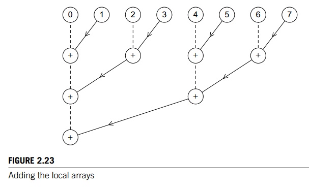
circle in the top row corresponds to a
process/thread. Between the first and the second rows, the odd-numbered
processes/threads make their loc bin cts available to the even-numbered
processes/threads. Then in the second row, the even-numbered processes/threads
add the new counts to their existing counts. Between the sec-ond and third rows
the process is repeated with the processes/threads whose ranks aren’t divisible
by four sending to those whose are. This process is repeated until
process/thread 0 has computed bin counts.
Related Topics