Engineering Analysis of Industrial Robots

        ENGINEERING   ANALYSIS  OF INDUSTRIAL   ROBOTS

In this section. we discuss two problem areas that are central to the operation of an industrial robot: (1) manipulator kinematics and (2) accuracy and repeatability with which the robot can position its end effector

          Introduction  to Manipulator  Kinematics

Manipulator kinematics is concerned with the position and orientation of the robot's end-of-arm. or the end effector attached to it as a function of time but without regard for the effects of force or mass. Of course, the mass of the manipulator's links and joints, not to mention the mass of the end effector and load being carried by the robot, will affect position and orientation as a function of time, but kinematic analysis neglects this effect. Our treatment of manipulator kinematics will be limited to the mathematical representation of the position and orientation of the robot's end-of-arm

Let us begin by defining terms, The robot manipulator consists of a sequence of joints and links. Let us name the joints J₁, J₂ and so on, starting with the joint closest to the base of the manipulator. Similarly, the links are identified as L₁,L₂ and so on, where L₁ is the output link of J₁,L₂ is the output link of J₂, and so on. Thus, the input link to J₂ is L₁ and the input link to J₁ is L₀. 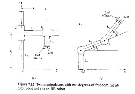The final link for a manipulator with n degrees-of-freedom (n joints) is Ln, and its position and orientation determine the position and orientation of the end effector attached to it. Figure 7.15 illustrates the joint and link identification method for two different manipulators, each having two joints. In Figure 7.15(a), both joints arc orthogonal types, so this is an  00 robot according to our notation scheme of Section 7.1.2. Let us define the values of the a joints as A₁ and A₂, where these values represent the positions

of the joints relative to their respective input links. Figure 7 .15(b) shows a two degree-of-freedom robot with configuration RR. Let us define the values of the two joints as the angles θ₁ and θ₂, where θ₁ is defined with respect to the horizontal .base. and θ₂ is defined relative to the direction of the input link to Joint le. as illustrated m our diagram

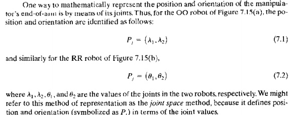
are the values of the joints in the two robots, respectively. We might refer to this method of representation as the joint space method, because it defines position and orientation (symbolized as P_I) in term, of the joint values. An alternative way to represent position is by the familiar Cartesian coordinate system, in robotics called the world space method. The origin of thc Cartesian coordinates in world space is usually located in the robot's base. The end-of-arm position Pw is defined in world space as

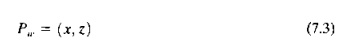
where x and z are the coordinates of point P_w. Only two axes are needed for our two-axis robots because the only positions that can be reached by the robots are in the x-z plane. For a robot with six joints operating in 3D space, the end-of-arm position and orientation Pu,can be defined as

where x, v, and z specify the Cartesian coordinates in world space (position) and a,,B,and X specify the angles of rotation of the three wrist joints (orientation).

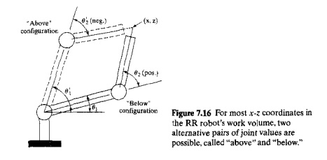
Notice that orientation cannot be independently established for our two robots in Figure 7.15. For the 00 manipulator, the end-of-arm orientation is always vertical; and for the RR manipulator, the orientation is determined by the joint angles θ1 and θ,. The reader will observe that the RR robot has two possible ways of reaching a given set of x and z coordinates, and so there are two alternative orientations of the endofarm that are possible for all xz values within the manipulator's reach except for those coordinate positions making up the outer circle of the work volume when θ2 is zero. The two alternative pairs of joint values are illustrated in Figure 7.16.

Forward and Backward Transformation for a Robot with Two Joints, Both the joint space and world space methods of defining position in the robot's space are important. The joint space method is important because the manipulator positions its end-of-arm by moving its Joints to certain values. The world space method is important because applications of the robot are defined in terms of points in space using the Cartesian coordinate system. What is needed is a means of mapping from one space method to the other.

Mapping from joint space to world space is called forward transformation, and converting from world space to joint space is called backward transformation.

The forward and backward transformations arc readily accomplished for the Cartesian coordinate robot of Figure 7,15(a), because the x and z coordinates correspond directly with the values of the joints, For the forward transformation,

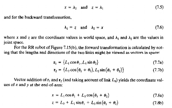
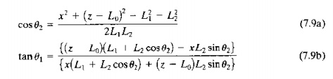
For the backward transformation, we are given the coordinate positions x and z in world space, and we must calculate the joint values that will provide those coordinate values. For our RR robot, we must first decide whether the robot will be positioned at the .r, z coordinates using an "above" or "below" configuration, as defined in Figure 7.16. Let us assume that the application calls for the below configuration, so that both θ. and θ₂ will take on positive values in our figure. Given the link values L1 and L2• the following equations can be derived for the two angles θ1 and θ2:

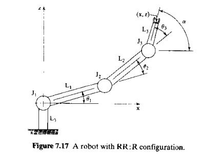
Forward and Backward Transformation for a Robot with Three Joints. Let us consider a manipulator with three degrees-of-freedom, all rotational, in which the third joint represents a simple wrist. The robot is a RR: R configuration, shown in Figure 7.17. We might argue that the arm-and-body (RR:) provides position of the end-of-arm, and the wrist (: R) provides orientation. The robot is still limited to the xz plane. Note that we have defined the origin of the axis system at the center of joint 1 rather than at the base of link 0, as in the previous RR robot of Figure 7.15(b). This was done to simplify the equations.

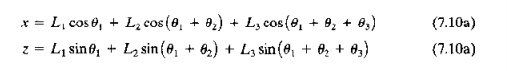
For the forward transformation, we can compute the x and z coordinates in a way similar to that used for the previous RR robot.

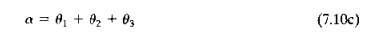
Let us define a as the orientation angle in Figure 7.17. It is the angle made by the wrist with the horizontal. It equals the algebraic sum of the three joint angles:

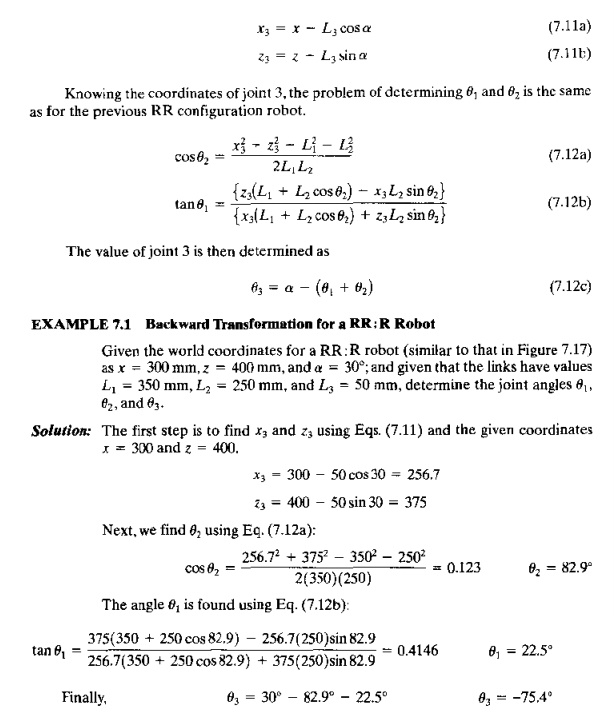
In the backward transformation. we are given the world coordinates x, z. and a, and we want to calculate the joint values OJ,92, and 9} that will achieve those coordinates. This is accomplished by first determining the coordinates of joint 3 (x3 and Z3 as shown in Figure 7.17). The coordinates are

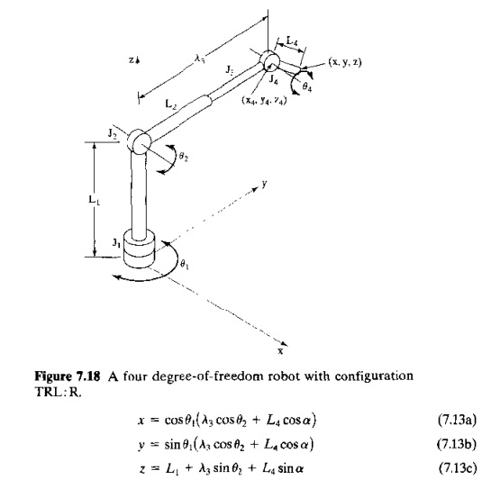
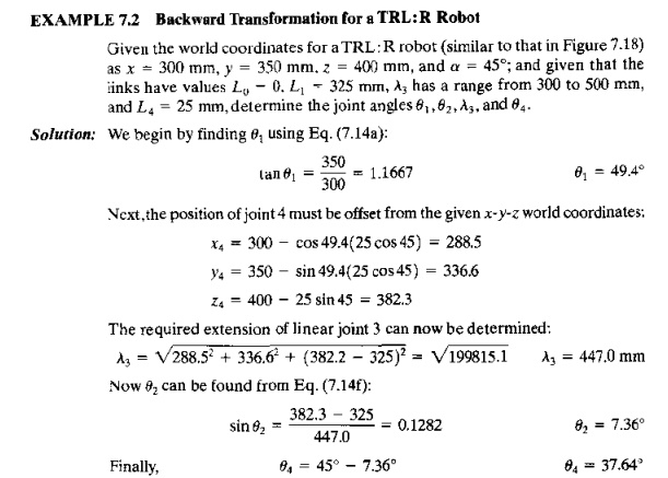
A Four-Jointed Robot in Three Dimensions. Most robots possess a work volume with three dimensions. Consider the fourdegreeoffreedom robot in Figure 7.18. Its configuration is TRL: R. Joint 1 (type T) provides rotation about the z axis, Joint 2 (type R) provides rotation about a horizontal axis whose direction is determined by joint 1. Joint 3 (type L) is a piston that allows linear motion in a direction determined by joints 1 and 2 And joint 4 (type R)

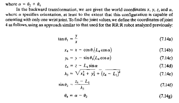
In the backward transformation, we are given the world coordinates .r, y, e. and a, where a specifies orientation, at least to the extent that this configuration is capable of orienting with only one wrist joint. To find the joint values, we define the coordinates of joint 4 as follows, using an approach similar to that used for the RR:R robot analyzed previously:

Homogeneous Transformations for Manipulator Kinematics. Each of the previous manipulators required its own individual analysis, resulting in its own set of trigonometric equations, to accomplish the forward and backward transformations. There is a general approach for solving the manipulator kinematic equations based on homogeneous transformations. Here we briefly describe the approach to make the reader aware of its availability. For those who are interested in homogeneous transformations for robot kinematics, more complete treatments of the topic are presented in several of our references, including Craig [3], Groover et al. [6], and Paul [9].

The homogeneous transformation approach utilizes vector and matrix algebra to define the joint and link positions and orientations with respect to a fixed coordinate system (world space). The end-of-arm is defined by the following 4 x 4 matrix:

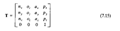
where T consists of four column vectors representing the position and orientation of the end-of-arm or end effector of the robot, as illustrated in Figure 7.19, The vector p defines the position coordinates of the end effector relative to the world x yz coordinate system The vectors a, 0, and n define the orientation of the end effector. The a vector, called the approach vector, points in the direction of the end effector, The 0 vector, or orientation

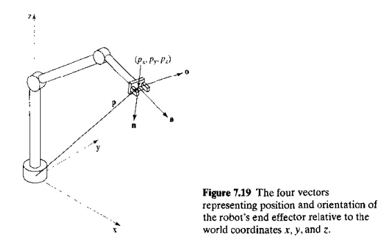
vector, specifies the side-to-side direction of the end effector. For a gripper, this is in the direction from one fingertip to the opposite fingertip. The II vector is the normal vector, which is perpendicular to a and o. Together, the vectors a, 0, and D constitute the coordinate axes of the tool coordinate system (Section 7.6.1).

A homogeneous transformation is a 4 x 4 matrix used to define the relative translation and rotation between coordinate systems in three-dimensional space. In manipulator kinematics, calculations based on homogeneous transformations are used to establish the geometric relationships among links of the manipulator. For example, let Ai = a 4 x 4 matrix that defines the position and orientation of link 1 with respect to the world coordinate axis system. Similarly, A2 = a 4 x 4 matrix that defines the position and orientation of the link 2 with respect to link 1.Then the position and orientation of link 2 with respect to the world coordinate system (call it T2) is given by:

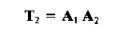
where T2 might represent the position and orientation of the end-of-arm (end of link 2) of a manipulator with two joints: and Al and A2 define the changes in position and orientation resulting from the actuations of joints I and 2 on links 1 and 2, respectively.

This approach can be extended to manipulators with more than two links. In general, the position and orientation of the end-of-arm or end effector can be determined as the product of a series uf homogeneous transformations, usually one transformation for each joint-link combination of the manipulator, These homogeneous transformations mathematically define the rotations and translations that are provided by the manipulator's joints and links. For the four-jointed robot analyzed earlier, the tool coordinate system (position and orientation of the end effector) might be represented relative to the world coordinate system as:

where T = the transformation matrix defining the tool coordinate system, as defined in Eq. (7.15); and A, = transformation matrices (4 x 4) for each of the four links of the manipulator.

       Accuracy   and  Repeatability

The capacity of the robot to position and orient the end of its wrist with  accuracy and repeatability is an Important control attribute in nearly all industrial applications. Some assembly applications require that objects be located with a precision of 0.05 mm (0.002 in) Other applications, such as spot welding, usually require accuracies of 0.51.0 mm (0.0200.040 in). Let us examine the question of how a robot is able to move its various joints to achieve accurate and repeatable positioning. There are several terms that must be defined in the context of this discussion: (1) control resolution, (2) accuracy, and (3) repeatability.

These terms have the same basic meanings in robotics that they have in NC. In robotics. the characteristics are defined at the end of the wrist and in the absence of any end effector attached at the wrist.

Control resolution refers to the capability of the robot's controller and positioning system to divide the range of the joint into closely spaced points that can be identified by the controller. These are called addressable points because they represent locations to which the robot can be commanded to move. Recall from Section 6.6.3 that the capability to divide the range into addressable points depends on two factors: (1) limitations of the electromechanical components that make up each joint-link combination and (2) the controller's bit storage capacity for that joint.

If the joint-link combination consists of a leadscrew drive mechanism, as in the case of an NC positioning system, then the methods of Section 6.6.3 can be used to determine the control resolution. We identified this electromechanical control resolution as CR10 Unfortunately, from our viewpoint of attempting to analyze the control resolution of the robot manipulator, there is a much wider variety of joints used in robotics than in NC machine tools. And it is not possible to analyze the mechanical details of all of the types here. Let it suffice to recognize that there is a mechanical limit on the capacity to divide the range of each joint-link system into addressable points, and that this limit is given by CR₁.

The second limit on control resolution is the bit storage capacity of the controller. If B = the number of bits in the bit storage register devoted to a particular joint, then the number of addressable points in that joint's range of motion is given by 2^B• The control resolution is therefore defined as the distance between adjacent addressable points.This can be determined as

where CR2 = control resolution determined by the robot controller; and R = range of the joint-link combination, expressed in linear or angular units, depending on whether the joint provides a linear motion (joint types L or 0) or a rotary motion (joint types R, T, or V). The control resolution of each joint-link mechanism will be the maximum of CRj and CR2; that is,

In our discussion of control resolution for NC (Section 6.6.3), we indicated that it is desirable for CR₂<=CRj, which means that the limiting factor in determining control resolution is the mechanical system, not the computer control system. Because the mechanical structure of a robot manipulator is much less rigid than that of a machine tool, the control resolution for each joint of a robot will almost certainly be determined by mechanical factors (CR,).

Similar to the case of an NC positioning system, the ability of a robot manipulator to position any given joint-link mechanism at the exact location defined by an addressable point is limited by mechanical errors in the joint and associated links. The mechanical errors arise from such factors as gear backlash, link deflection, hydraulic fluid leaks, and various other sources that depend on the mechanical construction of the given joint-link combination. If we characterize the mechanical errors by a normal distribution, as we did in Section 6,6.3, with mean /L at the addressable point and standard deviation 0" characterizing the magnitude of the error dispersion. then accuracy and repeatability for the axis can he defined.

Repeatability is the easier term to define. Repeatability is a measure of the robot's ability to position its end-of wrist at a previously taught point in the work volume. Each time the robot attempts to return to the programmed point it will return to a slightly different position. Repeatability errors have as their principal source the mechanical errors previously mentioned. Therefore, as in NC, for a single joint-link mechanism,

where  σ = standard      deviation     of the error  distribution,

Accuracy is a measure of the robot's ability to position the end of its wrist at a desired location in the work volume. For a single axis, using the same reasoning used to define ac. curacy in our discussion of NC, we have

where    CR=control      resolution   from Eq. (7.18).

The terms control resolution, accuracy, and repeatability are illustrated in Figure 6.29 of the previous chapter fur one axis that is linear. For a rotary joint, these parameters can be conceptualized as either an angular value of the joint itself or an arc length at the end of the joint's output link.

EXAMPLE    7.3 Control Resolution,      Accuracy, and Repeatability in Robotic  Arm Joint

One of the joints of a certain industrial robot has a type L joint with a range of 0.5 rn. The bit storage capacity of the robot controller is 10 bits for this joint. The mechanical errors form a normally distributed random variable about a given taught point. The mean of the distribution is zero and the standard deviation is 0,06 mm in the direction of the output link of the joint. Determine the control resolution (CR1), accuracy, and repeatability for this robot joint.

Solution: The number of addressable points in the joint range is 2¹⁰ = 1024. The control resolution is therefore

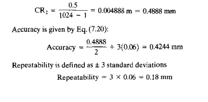
Our definitions of control resolution, accuracy, and repeatability have been depicted using a single joint or axis. To be of practical value, the accuracy and repeatability of a robot manipulator should include the effect of all of the joints, combined with the effect of their mechanical errors. For a multiple degree of freedom robot, accuracy and repeatability will vary depending on where in the work volume the end-of-wrist is positioned. The reason for this is that certain joint combinations will tend to magnify the effect of the control resolution and mechanical errors. For example. for a polar configuration robot (TRL) with its linear joint fully extended, any errors in the R or T joints will be larger than when the linear joint is fully retracted.

Robots move in three-dimensional space, and the distribution of repeatability errors is therefore three-dimensional. In 3D, we can conceptualize the normal distribution as a sphere whose center (mean) is at the programmed point and whose radius is equal to three standard deviations of the repeatability error distribution. For conciseness, repeatability is usually expressed in terms of the radius of the sphere; for example. ±1.0 mm (±O.040 in). Some of today's small assembly robots have repeatability values as low as ±0.05 mm (±O.OO2 in).

In reality, the shape of the error distribution will not be a perfect sphere in three dimensions. In other words, the errors will not be isotropic. Instead, the radius will vary because the associated mechanical errors will be different in certain directions than in others, The mechanical arm of a robot is more rigid in certain directions, and this rigidity influences the errors. Also, the so called sphere will not remain constant in size throughout the robot's work volume, As with spatial resolution, it will be affected by the particular combination of joint positions of the manipulator. In some regions of the work volume, the repeatability errors win be larger than in other regions.

Accuracy and repeatability have been defined above as static parameters of the manipulator. However, these precision parameters are affected by the dynamic operation of the robot. Such characteristics as speed, payload, and direction of approach will affect the robot's accuracy and repeatability.