Wide-Band FM

WIDE-BAND FM:

s(t) = ACcos(2πfct + φ(t)

Finding its FT is not easy:ϕ(t) is inside the cosine.

To analyze the spectrum, we use complex envelope.

s(t) can be written as: Consider single tone FM: s(t) =ACcos(2πfct + βsin2πfm(t))

Wideband FM is defined as the situation where the modulation index is above 0.5. Under these circumstances the sidebands beyond the first two terms are not insignificant. Broadcast FM stations use wideband FM, and using this mode they are able to take advantage of the wide bandwidth available to transmit high quality audio as well as other services like a stereo channel, and possibly other services as well on a single carrier.

The bandwidth of the FM transmission is a means of categorising the basic attributes for the signal, and as a result these terms are often seen in the technical literature associated with frequency modulation, and products using FM. This is one area where the figure for modulation index is used.

^ü   GENERATION OF WIDEBAND FM SIGNALS:

Indirect Method for Wideband FM Generation:

Consider the following block diagram

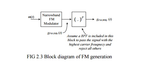
A narrowband FM signal can be generated easily using the block diagram of the narrowband FM modulator that was described in a previous lecture. The narrowband FM modulator generates a narrowband FM signal using simple components such as an integrator (an OpAmp), oscillators, multipliers, and adders. The generated narrowband FM signal can be converted to a wideband FM signal by simply passing it through a non–linear device with power P. Both the carrier frequency and the frequency deviation Df of the narrowband signal are increased by a factor P. Sometimes, the desired increase in the carrier frequency and the desired increase in Df are different. In this case, we increase Df to the desired value and use a frequency shifter (multiplication by a sinusoid followed by a BPF) to change the carrier frequency to the desired value.

^ü   System 1:

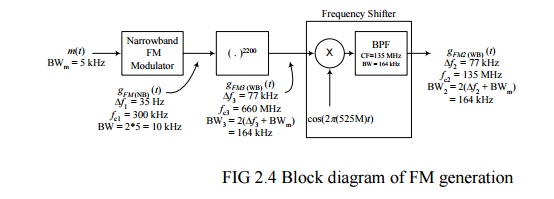
In this system, we are using a single non–linear device with an order of 2200 or multiple devices with a combined order of 2200. It is clear that the output of the non–linear device has the correct

Df but an incorrect carrier frequency which is corrected using a the frequency shifter with an oscillator that has a frequency equal to the difference between the frequency of its input signal and the desired carrier frequency. We could also have used an oscillator with a frequency that is the sum of the frequencies of the input signal and the desired carrier frequency. This system is characterized by having a frequency shifter with an oscillator frequency that is relatively large.

 ü   System 2:

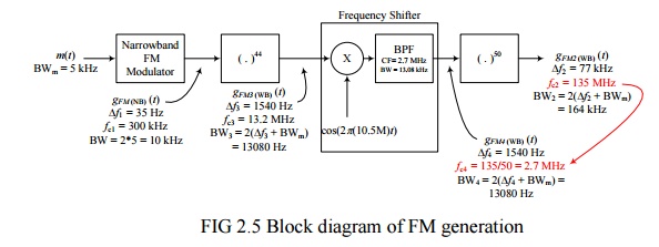
In this system, we are using two non–linear devices (or two sets of non–linear devices) with orders 44 and 50 (44*50 = 2200). There are other possibilities for the factorizing 2200 such as 2*1100,4*550,8*275,10*220.. Depending on the available components, one of these factorizations may be better than the others. In fact, in this case, we could have used the same factorization but put 50 first followed by 44. We want the output signal of the overall system to be as shown in the block diagram above, so we have to insure that the input to the non–linear device with order 50 has the correct carrier frequency such that its output has a carrier frequency of 135 MHz. This is done by dividing the desired output carrier frequency by the non–linearity order of 50, which gives 2.7 Mhz. This allows us to figure out the frequency of the require oscillator which will be in this case either 13.2–2.7 = 10.5 MHz or 13.2+2.7 = 15.9 MHz. We are generally free to choose which ever we like unless the available components dictate the use of one of them and not the other. Comparing this system with System 1 shows that the frequency of the oscillator that is required here is significantly lower (10.5 MHz compared to 525 MHz), which is generally an advantage.

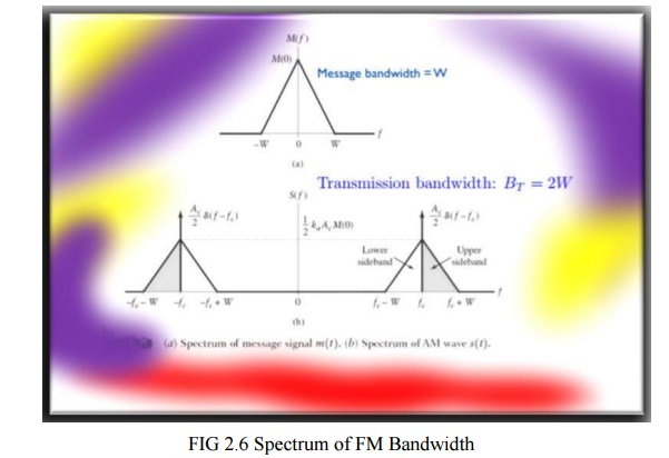
TRANSMISSION BANDWIDTH: