Unicast Routing Protocols

Unicast Routing Protocols

A routing table can be either static or dynamic. A static table is one with manual entries. A dynamic table, on the other hand, is one that is updated automatically when there is a change somewhere in the internet. Today, an internet needs dynamic routing tables. The tables need to be updated as soon as there is a change in the internet. For instance, they need to be updated when a router is down, and they need to be updated whenever a better route has been found.

1. Optimization

A router receives a packet from a network and passes it to another network. A router is usually attached to several networks. One approach is to assign a cost for passing through a network. We call this cost a metric. However, the metric assigned to each network depends on the type of protocol. Some simple protocols, such as the Routing Information Protocol (RIP), treat all networks as equals. The cost of passing through a network is the same; it is one hop

count. So if a packet passes through 10 networks to reach the destination, the total cost is 10 hop counts.

2. Intra- and Inter-domain Routing

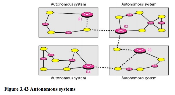
An internet can be so large that one routing protocol cannot handle the task of updating the routing tables of all routers. For this reason, an internet is divided into autonomous systems. An autonomous system (AS) is a group of networks and routers under the authority of a single administration. Routing inside an autonomous system is referred to as intradomain routing. Routing between autonomous systems is referred to as interdomain routing

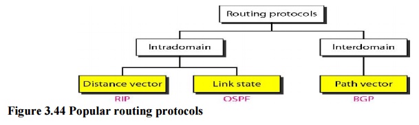
Several intradomain and interdomain routing protocols are in use.

O Two intradomain routing protocols: Distance vector and link state.

O One interdomain routing protocol: path vector.

Routing Information Protocol (RIP) is an implementation of the distance vector protocol. Open Shortest Path First (OSPF) is an implementation of the link state protocol. Border Gateway Protocol (BGP) is an implementation of the path vector protocol.

3. Distance Vector Routing

In distance vector routing, the least-cost route between any two nodes is the route with minimum distance. In this protocol, as the name implies, each node maintains a vector (table) of minimum distances to every node. The table at each node also guides the packets to the desired node by showing the next stop in the route (next-hop routing).

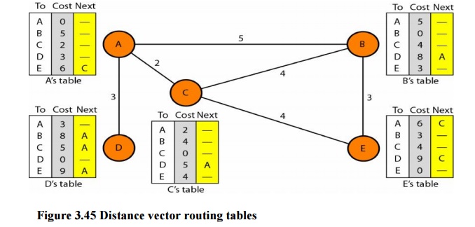
The table for node A shows how we can reach any node from this node. For example, our least cost to reach node E is 6. The route passes through C.

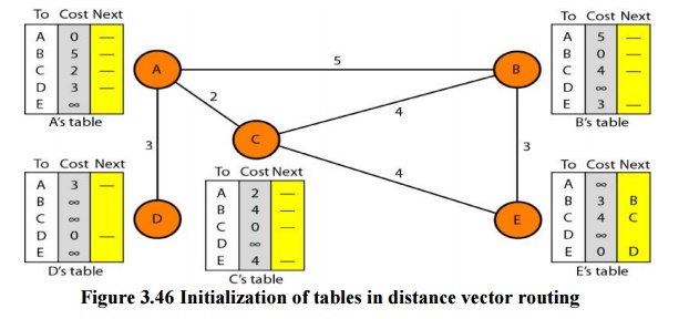
Initialization

The tables in Figure 3.45 are stable; each node knows how to reach any other node and the cost. At the beginning, however, this is not the case. Each node can know only the distance between itself and its immediate neighbors, those directly connected to it. So for the moment, we assume that each node can send a message to the immediate neighbors and find the distance between itself and these neighbors. The distance for any entry that is not a neighbor is marked as infinite (unreachable).

Sharing

The whole idea of distance vector routing is the sharing of information between neighbors. Although node A does not know about node E, node C does. So if node C shares its routing table with A, node A can also know how to reach node E. On the other hand, node C does not know how to reach node D, but node A does. If node A shares its routing table with node C, node C also knows how to reach node D. In other words, nodes A and C, as immediate neighbors, can improve their routing tables if they help each other.

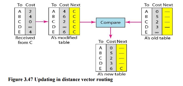
Updating

When a node receives a two-column table from a neighbor, it needs to update its routing table. Updating takes three steps:

1. The receiving node needs to add the cost between itself and the sending node to each value in the second column. The logic is clear. If node C claims that its distance to a destination is x mi, and the distance between A and C is y mi, then the distance between A and that destination, via C, is x + y mi.

2. The receiving node needs to add the name of the sending node to each row as the third column if the receiving node uses information from any row. The sending node is the next node in the route.

3. The receiving node needs to compare each row of its old table with the corresponding row of the modified version of the received table.

a)        If the next-node entry is different, the receiving node chooses the row with the smaller cost. If there is a tie, the old one is kept.

b)       If the next-node entry is the same, the receiving node chooses the new row. For example, suppose node C has previously advertised a route to node X with distance 3.

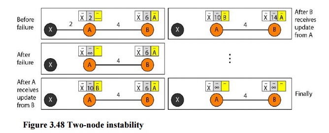
Two-Node Loop Instability

A problem with distance vector routing is instability, which means that a network using this protocol can become unstable. To understand the problem, let us look at the scenario depicted.

Defining Infinity The first obvious solution is to redefine infinity to a smaller number, such as100. For our previous scenario, the system will be stable in less than 20 update s. As a matter of fact, most implementations of the distance vector protocol define the distance between each node to be I and define 16 as infinity. However, this means that the distance vector routing cannot be used in large systems. The size of the network, in each direction, cannot exceed 15 hops.

Split Horizon Another solution is called split horizon. In this strategy, instead of flooding thetable through each interface, each node sends only part of its table through each interface. If, according to its table, node B thinks that the optimum route to reach X is via A, it does not need to advertise this piece of information to A; the information has corne from A (A already knows). Taking information from node A, modifying it, and sending it back to node A creates the confusion. In our scenario, node B eliminates the last line of its routing table before it sends it to A. In this case, node A keeps the value of infinity as the distance to X.

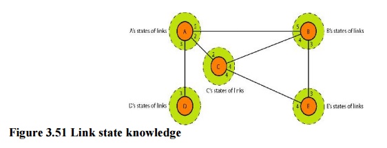
4. Link State Routing

Link state routing has a different philosophy from that of distance vector routing. In link state routing, if each node in the domain has the entire topology of the domain the list of nodes and links, how they are connected including the type, cost (metric), and condition of the links (up or down)-the node can use Dijkstra's algorithm to build a routing table.

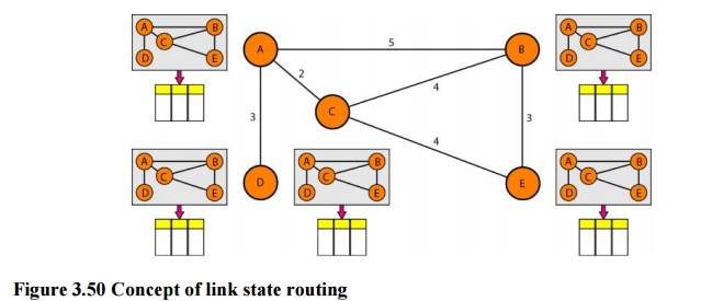
Figure 3.50 Concept of link state routing

The figure shows a simple domain with five nodes. Each node uses the same topology to create a routing table, but the routing table for each node is unique because the calculations are based on different interpretations of the topology. This is analogous to a city map. While each person may have the same map, each needs to take a different route to reach her specific destination

Building Routing Tables:

In link state routing, four sets of actions are required to ensure that each node has therouting table showing the least-cost node to every other node.

a) Creation of the states of the links by each node, called the link state packet (LSP).

b)Dissemination of LSPs to every other router, called flooding, in an efficient and  reliable way.

c) Formation of a shortest path tree for each node.

d)Calculation of a routing table based on the shortest path tree.

Types of Links

In OSPF terminology, a connection is called a link. Four types of links have been defined: point-to-point, transient, stub, and virtual.

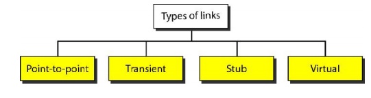
Figure 3.52 Types of links

A point-to-point link connects two routers without any other host or router in between. In other words, the purpose of the link (network) is just to connect the two routers. An example of this type of link is two routers connected by a telephone line or a T line. There is no need to assign a network address to this type of link. Graphically, the routers are represented by nodes, and the link is represented by a bidirectional edge connecting the nodes. The metrics, which are usually the same, are shown at the two ends, one for each direction. In other words, each router has only one neighbor at the other side of the link.

5. Path Vector Routing

Distance vector and link state routing are both intradomain routing protocols. They can be used inside an autonomous system, but not between autonomous systems. These two protocols are not suitable for interdomain routing mostly because of scalability. Both of these routing protocols become intractable when the domain of operation becomes large. Distance vector routing is subject to instability if there are more than a few hops in the domain of operation. Link state routing needs a huge amount of resources to calculate routing tables. It also creates heavy traffic because of flooding. There is a need for a third routing protocol which we call path vector routing.

Path vector routing proved to be useful for interdomain routing. The principle of path vector routing is similar to that of distance vector routing. In path vector routing, we assume that there is one node in each autonomous system that acts on behalf of the entire autonomous system.

Initialization

At the beginning, each speaker node can know only the reach ability of nodes inside its autonomous system

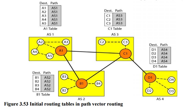
Figure 3.53 Initial routing tables in path vector routing

Node Al is the speaker node for AS1, B1 for AS2, C1 for AS3, and Dl for AS4. Node Al creates an initial table that shows Al to A5 are located in ASI and can be reached through it. Node B1 advertises that Bl to B4 are located in AS2 and can be reached through Bl. And so on.