Chapter: Fundamentals of Database Systems : The Relational Data Model and SQL : The Relational Algebra and Relational Calculus
Unary Relational Operations: SELECT and PROJECT
Unary Relational Operations: SELECT and PROJECT
1. The SELECT Operation
The SELECT operation is used to choose a subset of the tuples from a relation
that satisfies a selection condition.3
One can consider the SELECT
operation to be a filter that keeps
only those tuples that satisfy a qualifying condition. Alternatively, we can consider the SELECT operation to restrict the tuples in a relation to
only those tuples that satisfy the condition. The SELECT operation can also be visualized
as a horizontal partition of the
relation into two sets of tuples—those tuples that sat-isfy the condition and
are selected, and those tuples that do not satisfy the condition and are
discarded. For example, to select the EMPLOYEE tuples
whose department is 4, or
those whose salary is greater than $30,000, we can individually specify each of these two conditions with a SELECT operation as follows:
σDno=4(EMPLOYEE) σSalary>30000(EMPLOYEE)
In
general, the SELECT
operation is denoted by
σ<selection condition>(R)
where the
symbol σ (sigma) is used to denote the SELECT operator and the selec-tion
condition is a Boolean expression (condition) specified on the attributes of
relation R. Notice that R is generally a relational algebra expression whose result is a relation—the
simplest such expression is just the name of a database relation. The relation
resulting from the SELECT
operation has the same attributes as R.
The
Boolean expression specified in <selection condition> is made up of a
number of clauses of the form
<attribute
name> <comparison op> <constant value>
or
<attribute
name> <comparison op> <attribute name>
where
<attribute name> is the name of an attribute of R, <comparison op> is nor-mally one of the operators {=, <, ≤, >, ≥, ≠}, and <constant value> is
a constant value from the attribute domain. Clauses can be connected by the
standard Boolean oper-ators and, or, and not to form a general selection condition. For example, to select
the tuples for all employees who either work in department 4 and make over
$25,000 per year, or work in department 5 and make over $30,000, we can specify
the following SELECT
operation:
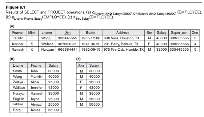
σ(Dno=4 AND Salary>25000) OR (Dno=5 AND Salary>30000)(EMPLOYEE)
The
result is shown in Figure 6.1(a).
Notice
that all the comparison operators in the set {=, <, ≤, >, ≥, ≠} can apply to attributes whose
domains are ordered values, such as
numeric or date domains. Domains of strings of characters are also considered
to be ordered based on the col-lating sequence of the characters. If the domain
of an attribute is a set of unordered
values, then only the comparison
operators in the set {=, ≠} can be used. An exam-ple of an unordered domain is the domain Color = { ‘red’, ‘blue’, ‘green’,
‘white’, ‘yel-low’, ...}, where no order is specified among the various colors.
Some domains allow additional types of comparison operators; for example, a
domain of character strings may allow the comparison operator SUBSTRING_OF.
In
general, the result of a SELECT
operation can be determined as follows. The <selection condition> is
applied independently to each individual
tuple t in R. This is done by
substituting each occurrence of an attribute Ai in the selection condition with its value in the
tuple t[Ai]. If the condition evaluates to TRUE, then tuple t is

selected. All the selected tuples appear
in the result of the SELECT operation.
The Boolean conditions AND, OR, and NOT have
their normal interpretation, as follows:
(cond1 AND cond2)
is TRUE if both (cond1) and (cond2) are TRUE; other-wise, it is FALSE.
(cond1 OR cond2)
is TRUE if either (cond1) or (cond2) or
both are TRUE;
otherwise, it is FALSE.
(NOT cond) is
TRUE if cond is FALSE; otherwise, it is FALSE.
The SELECT operator is unary; that is, it is applied to a single relation. Moreover, the
selection operation is applied to each
tuple individually; hence, selection condi-tions cannot involve more than
one tuple. The degree of the
relation resulting from a SELECT
operation—its number of attributes—is the same as the degree of R. The number of tuples in the resulting
relation is always less than or equal to
the number of tuples in R. That is, |σc (R)| ≤ |R| for any condition C. The fraction of tuples selected by a
selection condition is referred to as the selectivity
of the condition.
Notice
that the SELECT
operation is commutative; that is,
σ<cond1>(σ<cond2>(R)) = σ<cond2>(σ<cond1>(R))
Hence, a
sequence of SELECTs can be
applied in any order. In addition, we can always combine a cascade (or sequence) of
SELECT operations into a single SELECT operation with a conjunctive (AND) condition; that is,
σ<cond1>(σ<cond2>(...(σ<condn>(R)) ...)) = σ<cond1> AND<cond2> AND...AND <condn>(R)
In SQL,
the SELECT condition is typically specified
in the WHERE clause of a query. For example,
the following operation:
σDno=4 AND Salary>25000 (EMPLOYEE)
would
correspond to the following SQL query:
SELECT *
FROM EMPLOYEE
WHERE Dno=4 AND Salary>25000;
2. The PROJECT Operation
If we
think of a relation as a table, the SELECT
operation chooses some of the rows
from the table while discarding other rows. The PROJECT operation, on the other hand, selects certain columns from the table and discards the other columns. If we are
interested in only certain attributes of a relation, we use the PROJECT operation to project the relation over these
attributes only. Therefore, the result of the PROJECT operation can be visualized as a vertical partition of the relation into
two relations: one has the needed columns (attributes) and contains the result
of the operation, and the other contains the discarded columns. For example, to
list each employee’s first and last name and salary, we can use the PROJECT operation as follows:
πLname, Fname, Salary(EMPLOYEE)
The
resulting relation is shown in Figure 6.1(b). The general form of the PROJECT operation is
π<attribute list>(R)
where π (pi) is the symbol used to
represent the PROJECT
operation, and <attribute list> is the desired sublist of attributes from
the attributes of relation R. Again,
notice that R is, in general, a relational algebra expression whose
result is a relation, which in the simplest case is just the name of a database
relation. The result of the PROJECT operation
has only the attributes specified in <attribute list> in the
same order as
they appear in the list. Hence, its degree is equal to the number of attributes in <attribute list>.
If the
attribute list includes only nonkey attributes of R, duplicate tuples are likely to occur. The PROJECT operation removes any duplicate tuples, so the result of the PROJECT operation is a set of distinct
tuples, and hence a valid relation. This is
known as duplicate elimination. For example,
consider the following PROJECT operation:
πSex, Salary(EMPLOYEE)
The
result is shown in Figure 6.1(c). Notice that the tuple <‘F’, 25000>
appears only once in Figure 6.1(c), even though this combination of values
appears twice in the EMPLOYEE relation.
Duplicate elimination involves sorting or some other tech-nique to detect
duplicates and thus adds more processing. If duplicates are not elim-inated,
the result would be a multiset or bag of tuples rather than a set. This
was not permitted in the formal relational model, but is allowed in SQL (see Section
4.3).
The
number of tuples in a relation resulting from a PROJECT operation is always less than or equal to the number of tuples in R. If the projection list is a superkey
of R—that is, it includes some key of R—the resulting relation has the same number of tuples as R. Moreover,
π<list1> (π<list2>(R)) = π<list1>(R)
as long
as <list2> contains the attributes in <list1>; otherwise, the
left-hand side is an incorrect expression. It is also noteworthy that
commutativity does not hold on
PROJECT.
In SQL,
the PROJECT attribute list is specified in
the SELECT clause of a query. For example,
the following operation:
πSex, Salary(EMPLOYEE)
would
correspond to the following SQL query:
SELECT DISTINCT Sex, Salary
FROM EMPLOYEE
Notice
that if we remove the keyword DISTINCT from
this SQL query, then dupli-cates will not be eliminated. This option is not
available in the formal relational algebra.
3. Sequences of
Operations and the RENAME Operation
The
relations shown in Figure 6.1 that depict operation results do not have any
names. In general, for most queries, we need to apply several relational
algebra operations one after the other. Either we can write the operations as a
single relational algebra expression by
nesting the operations, or we can apply one operation at a time and create
intermediate result relations. In the latter case, we must give names to the
relations that hold the intermediate results. For example, to retrieve the
first name, last name, and salary of all employees who work in depart-ment
number 5, we must apply a SELECT and a PROJECT operation. We can write a single
relational algebra expression, also known as an in-line expression, as follows:
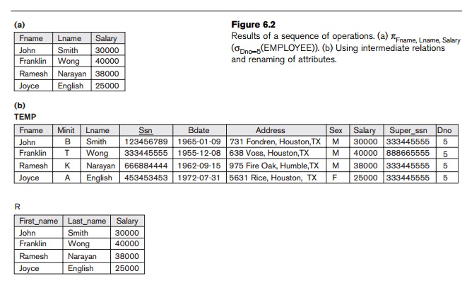
πFname, Lname, Salary(σDno=5(EMPLOYEE))
Figure
6.2(a) shows the result of this in-line relational algebra expression.
Alternatively, we can explicitly show the sequence of operations, giving a name
to each intermediate relation, as follows:
DEP5_EMPS ← σDno=5(EMPLOYEE)
RESULT ← πFname, Lname, Salary(DEP5_EMPS)
It is
sometimes simpler to break down a complex sequence of operations by specifying
intermediate result relations than to write a single relational algebra
expression. We can also use this technique to rename the attributes in the intermediate and

result
relations. This can be useful in connection with more complex operations such
as UNION and JOIN, as we shall see. To rename the
attributes in a relation, we simply list the new attribute names in
parentheses, as in the following example:
TEMP ← σDno=5(EMPLOYEE)
R(First_name, Last_name, Salary) ← πFname, Lname, Salary(TEMP)
These two
operations are illustrated in Figure 6.2(b).
If no
renaming is applied, the names of the attributes in the resulting relation of a
SELECT operation are the same as those
in the original relation and in the same
order.
For a PROJECT operation with no renaming, the
resulting relation has the same attribute names as those in the projection list
and in the same order in which they appear in the list.
We can
also define a formal RENAME
operation—which can rename either the relation name or the attribute names, or
both—as a unary operator. The general RENAME
operation
when applied to a relation R
of degree n is denoted by any of the following three forms:
ρS(B1,
B2, ..., Bn)(R) or ρS(R) or ρ(B1,
B2, ..., Bn)(R)
where the
symbol ρ (rho) is used to denote the RENAME operator, S is the new relation name, and B1, B2,
..., Bn are the new
attribute names. The first expression renames both the relation and its
attributes, the second renames the relation only, and the third renames the
attributes only. If the attributes of R
are (A1, A2, ..., An) in that order, then each Ai is renamed as Bi.
In SQL, a
single query typically represents a complex relational algebra expression.
Renaming in SQL is accomplished by aliasing using AS, as in the following example:
SELECT E.Fname AS First_name, E.Lname AS Last_name, E.Salary AS Salary
FROM EMPLOYEE AS E
WHERE E.Dno=5,
Related Topics