Chapter: Fundamentals of Database Systems : The Relational Data Model and SQL : The Relational Algebra and Relational Calculus
Binary Relational Operations: JOIN and DIVISION
Binary Relational Operations: JOIN and DIVISION
1. The JOIN Operation
The JOIN operation, denoted by ![]() , is used to combine related tuples from two rela-tions into single “longer” tuples.
This operation is very important for any relational database with more than a
single relation because it allows us to process relation-ships among relations.
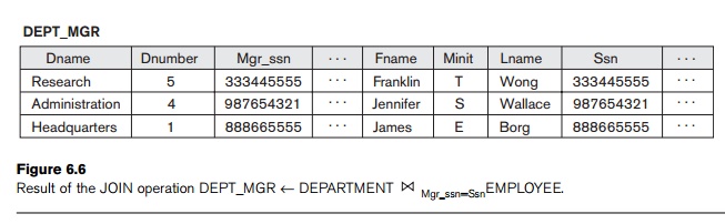
To illustrate JOIN, suppose that we want to retrieve the name of the manager of each
department. To get the manager’s name, we need to combine each department tuple
with the employee tuple whose Ssn value matches the Mgr_ssn value in the department tuple. We do this by using the JOIN operation and then projecting the result over
the necessary attributes, as follows:
, is used to combine related tuples from two rela-tions into single “longer” tuples.
This operation is very important for any relational database with more than a
single relation because it allows us to process relation-ships among relations.
To illustrate JOIN, suppose that we want to retrieve the name of the manager of each
department. To get the manager’s name, we need to combine each department tuple
with the employee tuple whose Ssn value matches the Mgr_ssn value in the department tuple. We do this by using the JOIN operation and then projecting the result over
the necessary attributes, as follows:
DEPT_MGR ← DEPARTMENT ![]() Mgr_ssn=Ssn EMPLOYEE
Mgr_ssn=Ssn EMPLOYEE
RESULT ← πDname,
Lname,
Fname(DEPT_MGR)
The first operation is illustrated in Figure 6.6. Note that Mgr_ssn is a foreign key of the DEPARTMENT relation
that references Ssn, the primary key of the EMPLOYEE relation.
This referential integrity constraint plays a role in having matching tuples in
the referenced relation EMPLOYEE.
The JOIN operation can be specified as a CARTESIAN PRODUCT
operation followed by a SELECT operation. However, JOIN is very important because it is used very frequently when specifying
database queries. Consider the earlier example illustrating CARTESIAN PRODUCT, which included the following sequence of operations:
EMP_DEPENDENTS ← EMPNAMES × DEPENDENT
ACTUAL_DEPENDENTS ← σSsn=Essn(EMP_DEPENDENTS)
These two operations can be replaced with a single JOIN operation as follows:
The result of the JOIN is a relation Q with n + m attributes Q(A1, A2, ..., An, B1, B2, ... , Bm) in that order; Q has one tuple for each combination of tuples—one from R and one from S—whenever the combination satisfies the join condition. This is the main difference between CARTESIAN PRODUCT and JOIN. In JOIN, only combina-tions of tuples satisfying the join condition appear in the result, whereas in the CARTESIAN PRODUCT all combinations of tuples are included in the result. The join condition is specified on attributes from the two relations R and S and is evaluated for each combination of tuples. Each tuple combination for which the join condition evaluates to TRUE is included in the resulting relation Q as a single combined tuple.
A general join condition is of the form
<condition> AND <condition> AND...AND <condition>
where each <condition> is of the form Ai θ Bj, Ai is an attribute of R, Bj is an attribute of S, Ai and Bj have the same domain, and θ (theta)
is one of the comparison operators {=, <, ≤, >, ≥, ≠}. A JOIN operation with such a general join condition is called a THETA JOIN. Tuples whose join attributes are NULL or for
which the join condition is FALSE do not appear in the result. In that sense, the JOIN operation does not necessarily
preserve all of the information in the participating relations, because tuples that do not get combined with
matching ones in the other relation do not appear in the result.
2. Variations of JOIN: The EQUIJOIN and NATURAL JOIN
The most
common use of JOIN involves
join conditions with equality comparisons only. Such a JOIN, where the only comparison
operator used is =, is called an EQUIJOIN. Both
previous examples were EQUIJOINs. Notice
that in the result of an EQUIJOIN we always
have one or more pairs of attributes that have identical values in every tuple. For example, in
Figure 6.6, the values of the attributes Mgr_ssn and Ssn are identical in every tuple of DEPT_MGR (the EQUIJOIN result) because the equality join condition specified
on these two attributes requires the
values to be identical in every
tuple in the result. Because one of each pair of attributes with identical values is superfluous, a new
operation called NATURAL JOIN—denoted
by * —was created to get rid of the second (superfluous) attribute
in an EQUIJOIN condition. The
standard definition of NATURAL JOIN requires
that the two join attributes (or each pair of join attributes) have the same
name in both relations. If this is not the case, a renaming operation is
applied first.
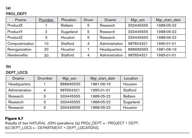
Suppose
we want to combine each PROJECT tuple
with the DEPARTMENT tuple
that controls the project. In the following example, first we rename the Dnumber attribute of DEPARTMENT to Dnum—so that it has the same name as
the Dnum attribute in
PROJECT—and then we apply NATURAL JOIN:
PROJ_DEPT ← PROJECT * ρ(Dname, Dnum, Mgr_ssn, Mgr_start_date)(DEPARTMENT)
The same
query can be done in two steps by creating an intermediate table DEPT as follows:
DEPT ← ρ(Dname, Dnum, Mgr_ssn, Mgr_start_date)(DEPARTMENT)
PROJ_DEPT ← PROJECT * DEPT
The
attribute Dnum is
called the join attribute for the NATURAL JOIN operation, because it is the
only attribute with the same name in both relations. The resulting relation is
illustrated in Figure 6.7(a). In the PROJ_DEPT
relation, each tuple combines a PROJECT tuple
with the DEPARTMENT tuple
for the department that controls the project, but only one join attribute value is kept.
If the
attributes on which the natural join is specified already have the same names in both
relations, renaming is unnecessary. For example, to apply a natural join on
the Dnumber attributes of
DEPARTMENT and DEPT_LOCATIONS, it is sufficient
to write
DEPT_LOCS ← DEPARTMENT * DEPT_LOCATIONS
The
resulting relation is shown in Figure 6.7(b), which combines each department
with its locations and has one tuple for each location. In general, the join
condition for NATURAL JOIN is
constructed by equating each pair of join
attributes that have the same name in the two relations and combining these
conditions with AND. There
can be a list of join attributes from each relation, and each corresponding
pair must have the same name.
A more
general, but nonstandard definition
for NATURAL JOIN is
Q ← R *(<list1>),(<list2>)S
In this
case, <list1> specifies a list of i
attributes from R, and <list2>
specifies a list of i attributes from
S. The lists are used to form
equality comparison conditions between pairs of corresponding attributes, and
the conditions are then ANDed
together. Only the list corresponding to attributes of the first relation R—<list1>— is kept in the result Q.
Notice
that if no combination of tuples satisfies the join condition, the result of a JOIN is an empty relation with zero tuples.
In general, if R
has nR tuples and S has nS
tuples,
the result of a JOIN
operation R![]() <join condition> S will have between zero and nR * nS tuples. The expected size
of the join result divided by the maximum size nR *
<join condition> S will have between zero and nR * nS tuples. The expected size
of the join result divided by the maximum size nR *
nS leads to a ratio called join
selectivity, which is a property of each join condition. If there is no join condition, all
combinations of tuples qualify and the JOIN
degen-erates into a CARTESIAN
PRODUCT, also
called CROSS PRODUCT or CROSS JOIN.
As we can
see, a single JOIN operation
is used to combine data from two relations so that related information can be
presented in a single table. These operations are also known as inner joins, to distinguish them from a
different join variation called outer
joins (see Section 6.4.4). Informally, an inner join is a type of match and com-bine operation defined
formally as a combination of CARTESIAN
PRODUCT and SELECTION. Note that sometimes a join may
be specified between a relation and
itself,
as we will illustrate in Section 6.4.3. The NATURAL
JOIN or EQUIJOIN opera-tion can also be specified
among multiple tables, leading to an n-way
join. For example, consider the following three-way join:
((PROJECT![]() Dnum=DnumberDEPARTMENT)
Dnum=DnumberDEPARTMENT)![]() Mgr_ssn=SsnEMPLOYEE)
Mgr_ssn=SsnEMPLOYEE)
This
combines each project tuple with its controlling department tuple into a single
tuple, and then combines that tuple with an employee tuple that is the
department manager. The net result is a consolidated relation in which each
tuple contains this project-department-manager combined information.
In SQL, JOIN can be realized in several different ways. The first method is to specify the <join conditions> in the WHERE clause, along with any other selection conditions. This is very common, and is illustrated by queries Q1, Q1A, Q1B, Q2, and Q8 in Sections 4.3.1 and 4.3.2, as well as by many other query examples in Chapters 4 and 5. The second way is to use a nested relation, as illustrated by queries Q4A and Q16 in Section 5.1.2. Another way is to use the concept of joined tables, as illustrated by the queries Q1A, Q1B, Q8B, and Q2A in Section 5.1.6. The construct of joined tables was added to SQL2 to allow the user to specify explicitly all the various types of joins, because the other methods were more limited. It also allows the user to clearly distinguish join conditions from the selection conditions in the WHERE clause.
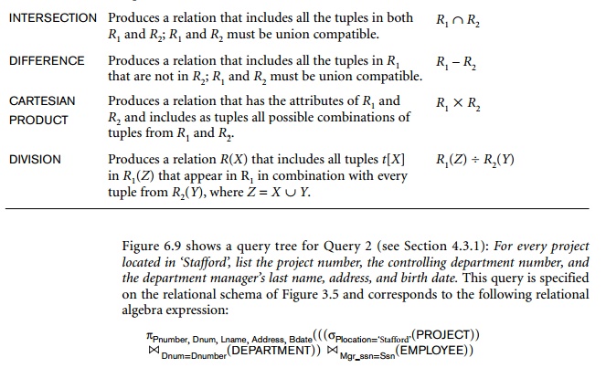
3. A Complete Set of
Relational Algebra Operations
It has
been shown that the set of relational algebra operations {σ, π, ∪, ρ, –, ×} is a complete set; that is, any of the other original relational algebra
operations can be expressed as a sequence of operations from this set.
For example, the INTERSECTION
operation can be expressed by using UNION and MINUS as follows:
R ∩ S ≡ (R ∪ S) – ((R – S) ∪ (S –
R))
Although,
strictly speaking, INTERSECTION is not
required, it is inconvenient to specify this complex expression every time we
wish to specify an intersection. As another example, a JOIN operation can be specified as a CARTESIAN PRODUCT fol-lowed by a SELECT operation, as we discussed:

Similarly, a NATURAL JOIN can be specified as a CARTESIAN PRODUCT preceded by RENAME and followed by SELECT and PROJECT operations. Hence, the various JOIN operations are also not strictly necessary for the expressive power of the rela-tional algebra. However, they are important to include as separate operations because they are convenient to use and are very commonly applied in database applications. Other operations have been included in the basic relational algebra for convenience rather than necessity. We discuss one of these—the DIVISION operation—in the next section.
4. The DIVISION
Operation
The DIVISION operation, denoted by ÷, is
useful for a special kind of query that sometimes occurs in database
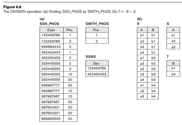
applications. An example is Retrieve the
names of employees who work on all the projects that ‘John Smith’
works on. To express this query
using the DIVISION
operation, proceed as follows. First, retrieve the list of project numbers that
‘John Smith’ works on in the intermediate relation
SMITH_PNOS:
SMITH
← σFname=‘John’
AND Lname=‘Smith’(EMPLOYEE)
SMITH_PNOS ← πPno(WORKS_ON![]() Essn=SsnSMITH)
Essn=SsnSMITH)
Next,
create a relation that includes a tuple <Pno, Essn> whenever the employee whose Ssn is Essn works on the project whose
number is Pno in the
intermediate relation SSN_PNOS:
SSN_PNOS ← πEssn, Pno(WORKS_ON)
Finally,
apply the DIVISION
operation to the two relations, which gives the desired employees’ Social
Security numbers:
SSNS(Ssn) ← SSN_PNOS ÷ SMITH_PNOS
RESULT ← πFname, Lname(SSNS * EMPLOYEE)
The
preceding operations are shown in Figure 6.8(a)
In
general, the DIVISION
operation is applied to two relations R(Z) ÷ S(X), where the attributes of R are a subset of the attributes of S; that is, X ⊆ Z. Let Y be the set of attributes of R
that are not attributes of S; that
is, Y = Z – X (and hence Z = X
∪ Y ). The
result of DIVISION is a
relation T(Y) that includes a tuple t if
tuples tR appear in R
with tR [Y] = t,
and with tR [X] = tS
for every tuple tS in S. This
means that, for a tuple t to appear
in the result T of the DIVISION, the values in t must appear in R in combination with every
tuple in S. Note that in the
formulation of the DIVISION
operation, the tuples in the denominator relation S restrict the numerator relation R by selecting those tuples in the result that match all values
present in the denomina-tor. It is not necessary to know what those values are
as they can be computed by another operation, as illustrated in the SMITH_PNOS relation in the above example.
Figure
6.8(b) illustrates a DIVISION
operation where X = {A}, Y
= {B}, and Z = {A, B}. Notice that the tuples (values) b1 and b4 appear in R in combination with all three
tuples in S; that is why they appear
in the resulting relation T. All
other values of B in R do not appear with all the tuples in S and are not selected: b2 does not appear with a2, and b3 does not appear with a1.
The DIVISION operation can be expressed as a
sequence of π, ×, and – operations as follows:
T1 ← πY(R)
T2 ← πY((S × T1) – R)
T ← T1 – T2
The DIVISION operation is defined for
convenience for dealing with queries that involve universal quantification (see Section 6.6.7) or the all condition. Most RDBMS implementations
with SQL as the primary query language do not directly implement division. SQL
has a roundabout way of dealing with the type of query illustrated above (see
Section 5.1.4, queries Q3A and Q3B). Table 6.1 lists the various
basic relational algebra operations we have discussed.
5. Notation for Query
Trees
In this
section we describe a notation typically used in relational systems to
represent queries internally. The notation is called a query tree or sometimes it is known as a query evaluation tree or query
execution tree. It includes the relational algebra operations being
executed and is used as a possible data structure for the internal
representation of the query in an RDBMS.
A query tree is a tree data structure
that corresponds to a relational algebra expression. It represents the input
relations of the query as leaf nodes
of the tree, and rep-resents the relational algebra operations as internal
nodes. An execution of the query tree consists of executing an internal node
operation whenever its operands (represented by its child nodes) are available,
and then replacing that internal node by the relation that results from
executing the operation. The execution terminates when the root node is
executed and produces the result relation for the query.

πPnumber, Dnum, Lname, Address, Bdate(((σPlocation=‘Stafford’(PROJECT))
![]() Dnum=Dnumber(DEPARTMENT))
Dnum=Dnumber(DEPARTMENT))![]() Mgr_ssn=Ssn(EMPLOYEE))
Mgr_ssn=Ssn(EMPLOYEE))
In Figure
6.9, the three leaf nodes P, D, and E represent the three relations PROJECT, DEPARTMENT, and
EMPLOYEE. The
relational algebra operations in the expression
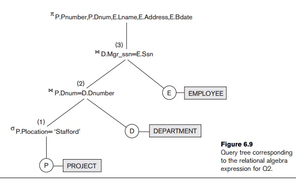
are
represented by internal tree nodes. The query tree signifies an explicit order
of execution in the following sense. In order to execute Q2, the node marked (1) in Figure
6.9 must begin execution before node (2) because some resulting tuples of
operation (1) must be available before we can begin to execute operation (2).
Similarly, node (2) must begin to execute and produce results before node (3)
can start execution, and so on. In general, a query tree gives a good visual
representation and understanding of the query in terms of the relational
operations it uses and is recommended as an additional means for expressing
queries in relational algebra. We will revisit query trees when we discuss
query processing and optimization in Chapter 19.
Related Topics