Types of Partial Differential Field Equations

Types of Partial Differential Field Equations

The world of Continuum Mechanics is very much a study of partial differential field equations (p.d.e.s) describing how vector and scalar components of tensors vary with position and how that field may vary with time. To make it easy, con-sider the general second order, linear p.d.e. in two variables:

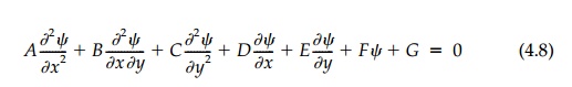
where _ is a general symbol for the field quantity and the two coordinates may be either space coordinates or one space coordinate plus time.

There are an infinite number of possible solutions to this general field equa-tion. The boundary conditions determine which particular solution is appro-priate. The solution _ (x,y) is a surface above and/or below the xy plane and the boundary is a specified curve in the xy plane. On this boundary, the boundary conditions are then, either:

a.  The height _ 'above' the boundary curve (the value of _) called the Dirichlet conditions, or

b.  The slope of the _ surface normal to the boundary curve (n · Grad _) called the Neumann condition, or

c.  Both, which is called the Cauchy boundary condition.

Three types of p.d.e.s are subsets of Equation (4.8) which are classified as shown in Table 4.1 along with their simplest examples. A unique and stable solution for each type of equation is possible only if the boundary conditions

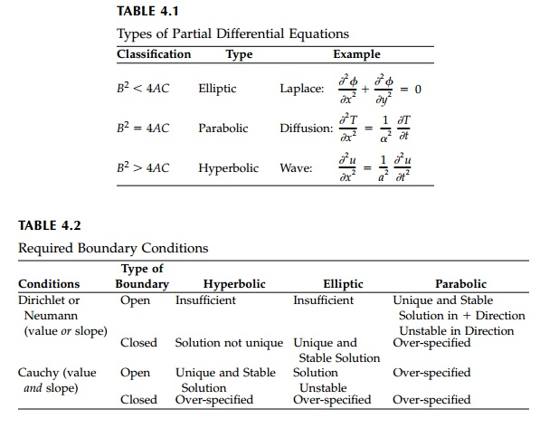
are specified properly* as shown in Table 4.2. For example, it is not possible to look backward in time** with a parabolic equation, which can describe such processes as the diffusion of a pollutant into a stream, thermal diffusion of tem-perature, or consolidation of saturated soil. The wave equation, on the other hand, which is hyperbolic, works equally well with negative or positive time.