Properties of Elliptic Equations

Properties of Elliptic Equations

Since we will deal primarily with elliptic equations, let us list a few important properties of these field equations and the associated boundary conditions:

a.  Boundary conditions must be Dirichlet or Neumann over a closed boundary. Part of the boundary may be at infinity (where the slope must be zero).

b.  The scalar function, , can have no maxima or minima inside the region where ² = 0. In other words, all maximums and mini-mums occur on the boundary of a Laplacian field. This is obviously a very important property for engineers who are particularly inter-ested in maximums and minimums.

c.  As a consequence, if the boundary conditions start the field increas-ing in a given direction, it has no choice but to continue increasing until it either goes to infinity (not a maximum, but a singularity) or the opposite boundary intervenes in time to stop it. That is why Cauchy conditions on an open boundary are not suitable.

However, elliptic equations are strongly damping (St. Venant's Prin-ciple). In fact, Laplace's equation is really a statement that the function and its slope at any point is the average of the values at neighboring points.

e.   Elliptic equations represent steady-state conditions. The field is what remains after the transient or particular solution in time disappears. Thus the other types of p.d.e.s (diffusion or wave equations) reduce to Laplace's equation when changes due to time damp out. Therefore, it is not surprising, perhaps, that elliptic equations are so common in the universe.*

d. Solutions to the Laplace equation come in pairs called conjugate harmonic functions. They obey the first-order Cauchy-Riemann con-ditions:

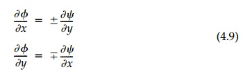
Thus taking the derivative of the first with respect to x and the second with respect to y and adding, gives ²= 0, or taking the derivative of the first with respect to y and the second with respect to x and subtracting gives ²= 0. One of the conjugate pair is often called the potential function and the other the stream function.

g.   The solution to Laplace's equation is a flow net where lines of equal  (contours of ) intersect lines of equal  (contours of ) at right angles. The Cauchy-Riemann conditions [Equation (4.9)] also require that the ratio of the adjacent sides of the resulting 'rectangles' remain constant (usually taken as 1.0 so that the flow net becomes a system of squares**). Actually  contours can be flow lines 'down' the  poten-tial 'hill' (the surface of  plotted above the xy plane) or  contours can be flow paths down the  potential hill. Constructing the flow net, which is an acquired skill is, in fact, a full graphical solution to Laplace's equation.

h.  The contours of equal (₁ + ₂) or mean stress _m, which we know now is either a potential or a stream function if the body force is zero or constant, are called isopachics.

Another elliptic equation which plays a major role in static elasticity is the nonhomogeneous Poisson's equation:

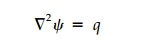
which arises when there is a source or sink q(x,y) in the field. For example, electric charge density, p, causes a negative concentration of the electric potential, V, so that ²V =-cp or a source of heat, Q, causes a concentration in temperature T so that ²T = KQ.

One way to visualize the Laplace and Poisson equations is to consider a perfectly elastic membrane in equilibrium under a uniform tension applied around its edge. If the edge lies entirely in a plane (perhaps tilted), the trivial solution  = ax + by + c results. If the boundary edge is now distorted into a nonlinear shape, the membrane is distorted also, but its height above the plane (x,y) still satisfies ² = 0. The tension straightens out all the 'bulges' introduced at the boundary and the displacement at any point equals the average of the neighboring points. One can also say that the membrane has arranged itself so that the average slope is a minimum. Thus the field condi-tion ²= 0 damps out all the edge values (St. Venant's principle) so that the membrane assumes a shape with the minimum stretching possible.

If now a distributed force, q(x,y), normal to the stretched membrane (which already satisfies 2= 0) is applied, the membrane will bulge. The Laplacian  is now proportional to this load per unit area, q, at any point. Shown in Figure 4.1 is a circular membrane loaded uniformly over the area 0 <= r <= 0.5 , and unloaded 0.5 <= r <= 1.0 . In the center region we have Poisson's equation

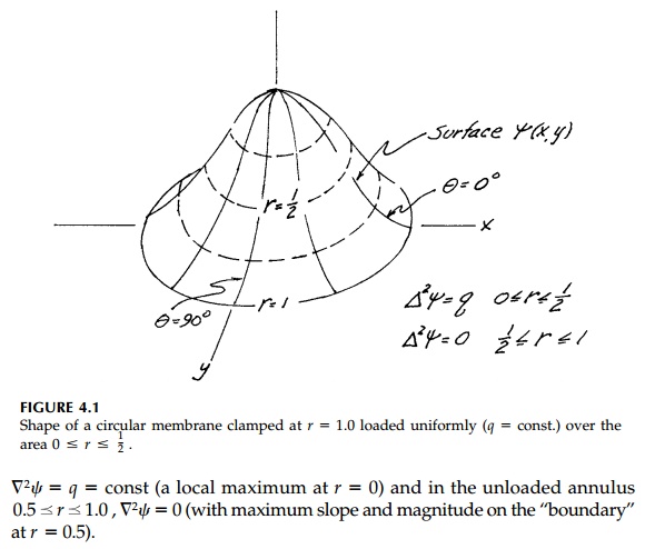
It is important to recognize that superposition holds for the Laplacian. If the boundary of the membrane in Figure 4.1 is now distorted, the new mem-brane shape will be simply  +  where  is the solution of 2= 0   for the membrane satisfying the distorted boundary. This is very useful in matching boundary conditions in that any amount of any solution of Laplace's equa-tion 2= 0   0 (homogeneous) can be added to  and still have a solution of 2 = q for the same particular q.