Chapter: Civil : Principles of Solid Mechanics : Strategies for Elastic Analysis and Design
The Conjugate Relationship Between Mean Stress and Rotation
The Conjugate
Relationship Between Mean Stress and Rotation
The first invariant of
the stress or strain tensor, the sum of the normal compo-nents, is harmonic for
a simply-connected domain and constant body forces. This in turn implies the
existence of a conjugate function, which must simi-larly be harmonic and also
invariant to linear tangent transformation.
From experience with
the significance of conjugate pairs in other potential fields, we might expect
a similar importance to be attached to the conjugate harmonic function in the
elastic continuum. This is not so. Occasionally pass-ing reference is made to a
conjugate relationship between elastic rotations and the mean stress or strain,
but the explicit statement of this correspon-dence is seldom presented.
This is probably
because in the standard formulation for simply-connected, two-dimensional
problems, the invariant elastic rotation, ![]() xy
, not correspond-ing directly to stress components, is neglected. The
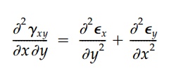
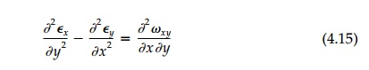
compatibility requirement is then expressed as:
xy
, not correspond-ing directly to stress components, is neglected. The
compatibility requirement is then expressed as:
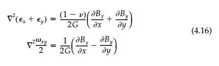
Finally by expressing
Equation (2.7) in terms of stresses from Equation (2.4) and combining with the
equilibrium Equation (2.45), the basic harmonic equations:
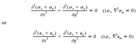
result whenever the
body forces Bx and By are negligible or
constant. The mean
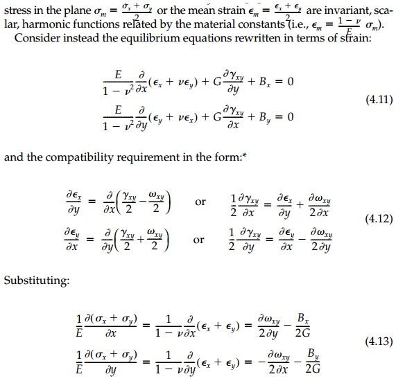
Thus, neglecting body
forces, we have the Cauchy-Riemann conditions directly and the conjugate
relationship between the elastic rotation of a differ-ential element and the
first invariant of the 2D stress tensor is established.
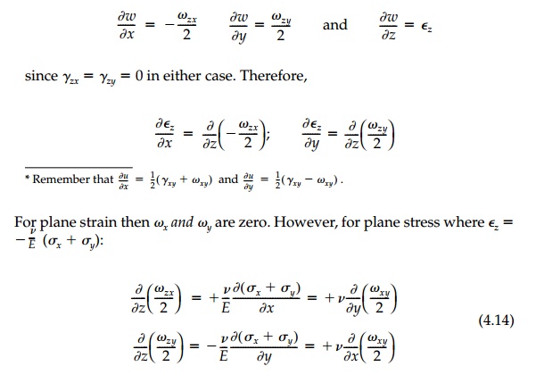
To determine elastic
rotations around the x and y axes associated with plane stress
and plane strain remember that:
Some general observations follow directly from these
equations:
1. For
an incompressible material ( v 0.5) in plane strain, Em
is zero and the displacements u and v themselves become conjugate
har-monic functions.
2. From
Equation (4.12) we can obtain the compatibility equation in its standard form
[Equation (2.7)] and derive a second independent relationship:
3. Both
the elliptic equations associated with Equation (4.13) are of similar form:
and are Laplacian
whenever the body forces are negligible or con-stant. In the event the body
forces are constant such as in a gravity field, Equation (4.13) can be reduced
to the Cauchy-Riemann con-ditions and direct solution achieved by a suitable
transformation. For example, if we define:
then from Equation
(4.13)
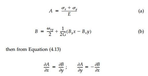
and
we can again solve for A and B by standard methods.
4. Direct
integration to determine displacements for plane strain (or plane stress in the
plane z = 0) is greatly
facilitated in that:
where now we can determine the rotation from the
stress field with Equation 4.13.
5. Finally
for the general 3D case, both the first invariant of the stress or strain
tensor:
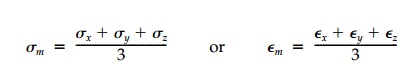
and the invariant mean
rotation of a volume element:
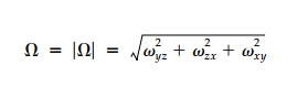
will
also clearly be Laplacian.
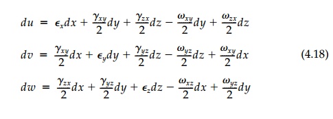
In general the
conjugate relationships are more complicated in three-dimensional situations.
Often, however, as is the case of plane stress [Equa-tion (4.14)] or where
there is a high degree of symmetry, the components of rotation can be
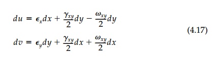
determined easily, in which case displacements can be found by direct integration
of the relative displacement equations:
Thus we see that,
without body forces, the elastic rotations times E are the conjugate
harmonic function to twice the mean stress and that these two sca-lar
invariants go 'hand-in-hand' throughout a structure, one controlling the other
in accordance with Laplace's equation. If we can solve for one, we have solved
for the other, and in that sense it is correct to neglect the rotations in that
they will come out of the solution for the stress (or strain) field of their
own accord.* This scalar part of the total tensor field giving the conjugate
har-monic invariants ![]() q
and
q
and ![]() xy
(or
xy
(or ![]() m
and
m
and ![]() in 3D) we shall call the 'isotropic field.' Only the
center of Mohr's Circle or, physically, pure volume change is involved.
in 3D) we shall call the 'isotropic field.' Only the
center of Mohr's Circle or, physically, pure volume change is involved.
Unfortunately it is
seldom possible to specify a complete set of proper boundary conditions in
terms of ![]() q
or
q
or ![]() xy
for problems in solid mechanics. For example, at most boundaries the tangential
normal stress is unknown, and only if the boundary is clamped will there be
zero rotation. Thus it is usu-ally not possible to solve for the
isotropic field independent of the deviatoric field.
xy
for problems in solid mechanics. For example, at most boundaries the tangential
normal stress is unknown, and only if the boundary is clamped will there be
zero rotation. Thus it is usu-ally not possible to solve for the
isotropic field independent of the deviatoric field.
Nevertheless,
flow nets are extremely useful:
1. To
depict the isotropic field so it can be understood once known.
2. Determine
the isotropic field if the boundary conditions can be found by other
methods such as photoelasticity which gives ![]() m
on the boundary directly.
m
on the boundary directly.
3. As
a conceptual tool for optimum design.
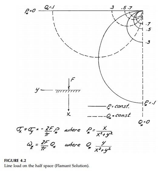
A number of isotropic
flow nets for important stress fields will be plotted in later chapters and
will be called for in chapter problems. Two examples are shown in Figures 4.2
and 4.3 which will be referred to later when the solutions to these important
problems are presented. In both these struc-tures, symmetry requires that
certain lines do not rotate, which simplifies the construction.
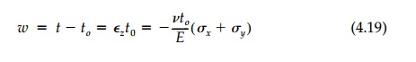
Interferometry provides
the best optical full-field method to see, in the lab-oratory, the
isopachics-contour lines of 'equal thickness'-which, by Equation (4.6), are
proportional to the mean stress. This is to say that, for plane stress, the
normal strain 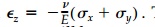 . Thus when a model is loaded,
the change in the thickness, t, will be
. Thus when a model is loaded,
the change in the thickness, t, will be
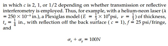
By interfering with the
wave front of light through or reflected off the unstressed model with the
wavefront from the stressed model, the change in thickness produces 'fringes'
of integer order N, proportional to w, with precision in
multiples of the wavelength of light, ![]() . More specifically
. More specifically
Until the advent of the
laser, interferometry was extremely expensive and not very successful even in
the hands of the best experimentalist. However, laser light is almost perfectly
monochromatic and, most importantly, coherent.
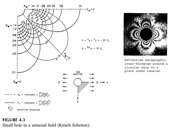
Thus, model surfaces
need not be flat since the reference (the unloaded) light beam can be captured
with a hologram. This makes the experimental deter-mination of the isotropic
stress field practical and the methodology continues to improve. A reflection
holographic interferogram is shown in Figure 4.3 for comparison to the
isopachics derived from the analytic solution.
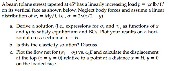
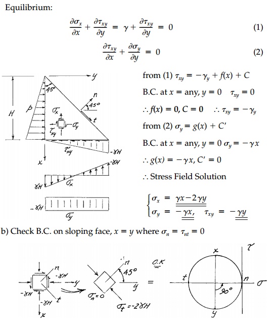
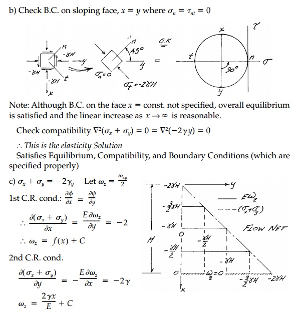
Example 4.1

Related Topics