Chapter: Distributed and Cloud Computing: From Parallel Processing to the Internet of Things : Distributed System Models and Enabling Technologies
Technologies for Network-Based Systems
TECHNOLOGIES FOR NETWORK-BASED SYSTEMS
With the concept of scalable
computing under our belt, it’s time to explore hardware,
software, and network technologies for distributed computing system design and
applications. In particular, we will focus on viable approaches to building
distributed operating systems for handling massive par-allelism in a
distributed environment.
1. Multicore CPUs and Multithreading
Technologies
Consider the growth of
component and network technologies over the past 30 years. They are crucial to
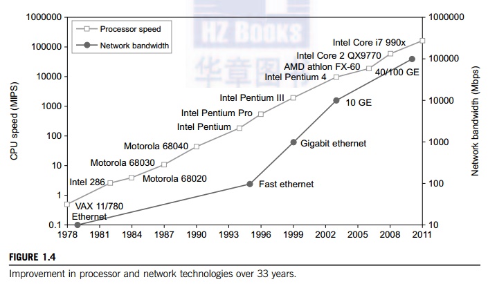
the development of HPC and HTC systems. In Figure 1.4, processor speed is
measured in millions
of instructions per second (MIPS) and network bandwidth is measured in megabits per second (Mbps) or gigabits per second (Gbps). The unit GE refers to 1 Gbps Ethernet bandwidth.
1.1
Advances in CPU Processors
Today, advanced CPUs or
microprocessor chips assume a multicore architecture with dual, quad, six, or
more processing cores. These processors exploit parallelism at ILP and TLP
levels. Processor speed growth is plotted in the upper curve in Figure 1.4
across generations of microprocessors or CMPs. We see growth from 1 MIPS for
the VAX 780 in 1978 to 1,800 MIPS for the Intel Pentium 4 in 2002, up to a
22,000 MIPS peak for the Sun Niagara 2 in 2008. As the figure shows, Moore’s law has proven to be pretty accurate in this
case. The clock rate for these processors increased from 10 MHz for the Intel
286 to 4 GHz for the Pentium 4 in 30 years.
However,
the clock rate reached its limit on CMOS-based chips due to power limitations.
At the time of this writing, very few CPU chips run with a clock rate exceeding
5 GHz. In other words, clock rate will not continue to improve unless chip
technology matures. This limitation is attributed primarily to excessive heat
generation with high frequency or high voltages. The ILP is highly exploited in
modern CPU processors. ILP mechanisms include multiple-issue superscalar
architecture, dynamic branch prediction, and speculative execution, among
others. These ILP techniques demand hardware and compiler support. In addition,
DLP and TLP are highly explored in graphics processing units (GPUs)
that adopt a many-core architecture with hundreds to thousands of simple cores.
Both
multi-core CPU and many-core GPU processors can handle multiple instruction
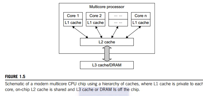
threads at different magnitudes today. Figure 1.5 shows the architecture of a
typical multicore processor. Each core is essentially a processor with its own
private cache (L1 cache). Multiple cores are housed in the same chip with an L2
cache that is shared by all cores. In the future, multiple CMPs could be built
on the same CPU chip with even the L3 cache on the chip. Multicore and
multi-threaded CPUs are equipped with many high-end processors, including the
Intel i7, Xeon, AMD Opteron, Sun Niagara, IBM Power 6, and X cell processors.
Each core could be also multithreaded. For example, the Niagara II is built
with eight cores with eight threads handled by each core. This implies that the
maximum ILP and TLP that can be exploited in Niagara is 64 (8 × 8 = 64). In 2011, the Intel Core i7 990x has
reported 159,000 MIPS execution rate as shown in the upper-most square in
Figure 1.4.
1.2
Multicore CPU and Many-Core GPU Architectures
Multicore CPUs may increase
from the tens of cores to hundreds or more in the future. But the CPU has
reached its limit in terms of exploiting massive DLP due to the aforementioned
memory wall problem. This has triggered the development of many-core GPUs with
hundreds or more thin cores. Both IA-32 and IA-64 instruction set architectures
are built into commercial CPUs. Now, x-86 processors have been extended to
serve HPC and HTC systems in some high-end server processors.
Many
RISC processors have been replaced with multicore x-86 processors and many-core
GPUs in the Top 500 systems. This trend indicates that x-86 upgrades will
dominate in data centers and supercomputers. The GPU also has been applied in
large clusters to build supercomputers in MPPs. In the future, the processor
industry is also keen to develop asymmetric or heterogeneous chip
mul-tiprocessors that can house both fat CPU cores and thin GPU cores on the
same chip.
1.3
Multithreading Technology
Consider in Figure 1.6 the
dispatch of five independent threads of instructions to four pipelined data
paths (functional units) in each of the following five processor categories,
from left to right: a
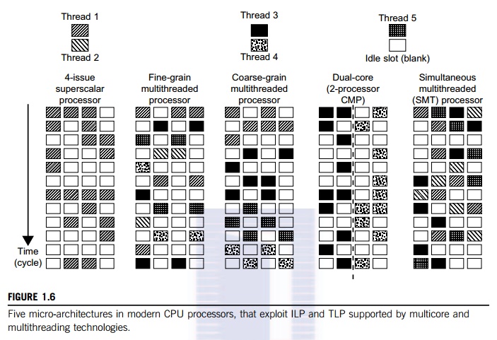
four-issue superscalar processor, a fine-grain multithreaded processor, a coarse-grain multi-threaded processor, a two-core CMP, and a simultaneous multithreaded (SMT) processor. The superscalar processor is single-threaded with four functional units. Each of the three multithreaded processors is four-way multithreaded over four functional data paths. In the dual-core processor, assume two processing cores, each a single-threaded two-way superscalar processor.
Instructions
from different threads are distinguished by specific shading patterns for
instruc-tions from five independent threads. Typical instruction scheduling
patterns are shown here. Only instructions from the same thread are executed in
a superscalar processor. Fine-grain multithread-ing switches the execution of
instructions from different threads per cycle. Course-grain multi-threading
executes many instructions from the same thread for quite a few cycles before
switching to another thread. The multicore CMP executes instructions from
different threads com-pletely. The SMT allows simultaneous scheduling of
instructions from different threads in the same cycle.
These execution patterns
closely mimic an ordinary program. The blank squares correspond to no available
instructions for an instruction data path at a particular processor cycle. More
blank cells imply lower scheduling efficiency. The maximum ILP or maximum TLP
is difficult to achieve at each processor cycle. The point here is to
demonstrate your understanding of typical instruction scheduling patterns in
these five different micro-architectures in modern processors.
2. GPU Computing to Exascale and
Beyond
A GPU is a graphics
coprocessor or accelerator mounted on a computer’s graphics card or video card. A GPU offloads
the CPU from tedious graphics tasks in video editing applications. The world’s first GPU, the GeForce 256, was marketed by
NVIDIA in 1999. These GPU chips can pro-cess a minimum of 10 million polygons
per second, and are used in nearly every computer on the market today. Some GPU
features were also integrated into certain CPUs. Traditional CPUs are
structured with only a few cores. For example, the Xeon X5670 CPU has six
cores. However, a modern GPU chip can be built with hundreds of processing
cores.
Unlike
CPUs, GPUs have a throughput architecture that exploits massive parallelism by
executing many concurrent threads slowly, instead of executing a single long
thread in a conven-tional microprocessor very quickly. Lately, parallel GPUs or
GPU clusters have been garnering a lot of attention against the use of CPUs
with limited parallelism. General-purpose
computing on GPUs, known as GPGPUs, have
appeared in the HPC field. NVIDIA’s CUDA model was for HPC using GPGPUs. Chapter 2 will discuss GPU
clusters for massively parallel computing in more detail [15,32].
2.1
How GPUs Work
Early GPUs functioned as
coprocessors attached to the CPU. Today, the NVIDIA GPU has been upgraded to
128 cores on a single chip. Furthermore, each core on a GPU can handle eight
threads of instructions. This translates to having up to 1,024 threads executed
concurrently on a single GPU. This is true massive parallelism, compared to
only a few threads that can be handled by a conventional CPU. The CPU is
optimized for latency caches, while the GPU is optimized to deliver much higher
throughput with explicit management of on-chip memory.
Modern
GPUs are not restricted to accelerated graphics or video coding. They are used
in HPC systems to power supercomputers with massive parallelism at multicore
and multithreading levels. GPUs are designed to handle large numbers of
floating-point operations in parallel. In a way, the GPU offloads the CPU from
all data-intensive calculations, not just those that are related to video processing.
Conventional GPUs are widely used in mobile phones, game consoles, embedded
sys-tems, PCs, and servers. The NVIDIA CUDA Tesla or Fermi is used in GPU
clusters or in HPC sys-tems for parallel processing of massive
floating-pointing data.
2.2
GPU Programming Model
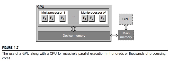
Figure 1.7 shows the
interaction between a CPU and GPU in performing parallel execution of
floating-point operations concurrently. The CPU is the conventional multicore
processor with limited parallelism to exploit. The GPU has a many-core
architecture that has hundreds of simple processing cores organized as
multiprocessors. Each core can have one or more threads. Essentially, the CPU’s floating-point kernel computation role is
largely offloaded to the many-core GPU. The CPU instructs the GPU to perform
massive data processing. The bandwidth must be matched between the on-board
main memory and the on-chip GPU memory. This process is carried out in NVIDIA’s CUDA programming using the GeForce 8800 or
Tesla and Fermi GPUs. We will study the use of CUDA GPUs in large-scale cluster
computing in Chapter 2.
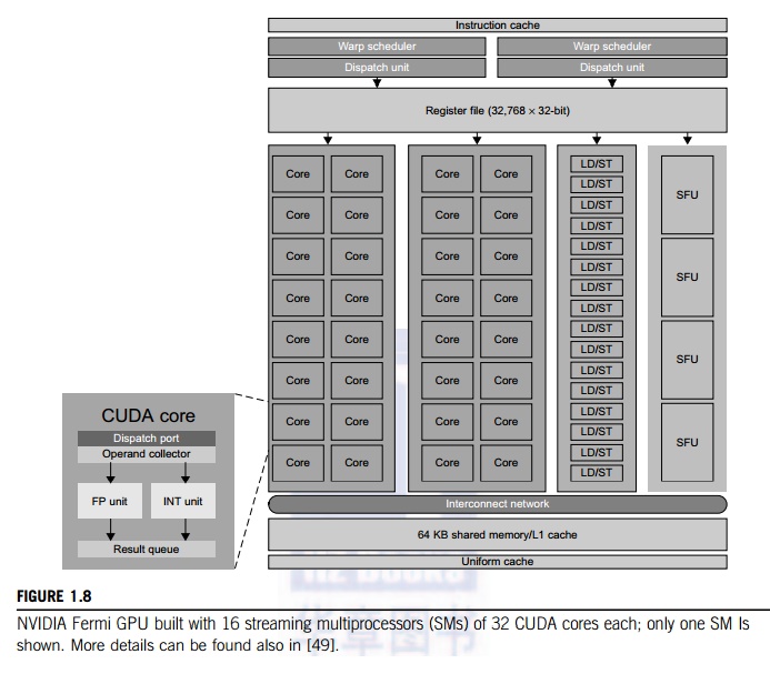
Example 1.1 The NVIDIA Fermi GPU Chip with 512
CUDA Cores
In November 2010, three of the five fastest
supercomputers in the world (the Tianhe-1a, Nebulae, and Tsubame) used large
numbers of GPU chips to accelerate floating-point computations. Figure 1.8
shows the architecture of the Fermi GPU, a next-generation GPU from NVIDIA.
This is a streaming multiprocessor (SM) module. Multiple SMs can be built on a
single GPU chip. The Fermi chip has 16 SMs implemented with 3 billion
transistors. Each SM comprises up to 512 streaming processors (SPs), known as
CUDA cores. The Tesla GPUs used in the Tianhe-1a have a similar architecture,
with 448 CUDA cores.
The
Fermi GPU is a newer generation of GPU, first appearing in 2011. The Tesla or
Fermi GPU can be used in desktop workstations to accelerate floating-point
calculations or for building large-scale data cen-ters. The architecture shown
is based on a 2009 white paper by NVIDIA [36]. There are 32 CUDA cores per SM.
Only one SM is shown in Figure 1.8. Each CUDA core has a simple pipelined
integer ALU and an FPU that can be used in parallel. Each SM has 16 load/store
units allowing source and destination addresses to be calculated for 16 threads
per clock. There are four special function units (SFUs) for executing
transcendental instructions.
All
functional units and CUDA cores are interconnected by an NoC (network on chip)
to a large number of SRAM banks (L2 caches). Each SM has a 64 KB L1 cache. The
768 KB unified L2 cache is shared by all SMs and serves all load, store, and
texture operations. Memory controllers are used to con-nect to 6 GB of off-chip
DRAMs. The SM schedules threads in groups of 32 parallel threads called warps.
In total, 256/512 FMA (fused multiply and add) operations can be done in
parallel to produce 32/64-bit floating-point results. The 512 CUDA cores in an
SM can work in parallel to deliver up to 515 Gflops of double-precision
results, if fully utilized. With 16 SMs, a single GPU has a peak speed of 82.4
Tflops. Only 12 Fermi GPUs have the potential to reach the Pflops performance.
In the
future, thousand-core GPUs may appear in Exascale (Eflops or 1018 flops) systems. This
reflects a trend toward building future MPPs with hybrid architectures of both
types of processing chips. In a DARPA report published in September 2008, four
challenges are identified for exascale computing: (1) energy and power, (2)
memory and storage, (3) concurrency and locality, and (4) system resiliency.
Here, we see the progress of GPUs along with CPU advances in power
efficiency, performance, and programmability [16]. In Chapter 2, we will discuss the use of GPUs to build large clusters.
2.3
Power Efficiency of the GPU
Bill Dally of Stanford
University considers power and massive parallelism as the major benefits of
GPUs over CPUs for the future. By extrapolating current technology and computer
architecture, it was estimated that 60 Gflops/watt per core is needed to run an
exaflops system (see Figure 1.10). Power constrains what we can put in a CPU or
GPU chip. Dally has estimated that the CPU chip consumes about 2
nJ/instruction, while the GPU chip requires 200 pJ/instruction, which is 1/10
less than that of the CPU. The CPU is optimized for latency in caches and
memory, while the GPU is optimized for throughput with explicit management of
on-chip memory.
Figure 1.9 compares the CPU
and GPU in their performance/power ratio measured in Gflops/ watt per core. In
2010, the GPU had a value of 5 Gflops/watt at the core level, compared with
less
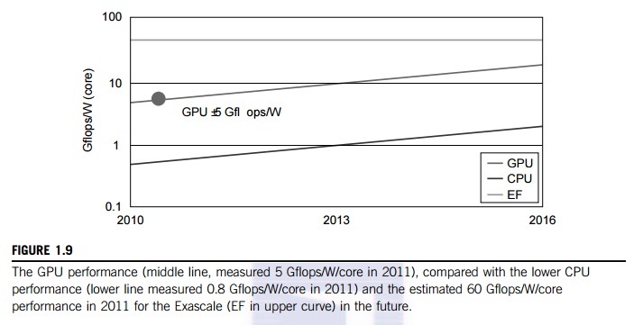
than 1 Gflop/watt per CPU
core. This may limit the scaling of future supercomputers. However, the GPUs
may close the gap with the CPUs. Data movement dominates power consumption. One
needs to optimize the storage hierarchy and tailor the memory to the
applications. We need to promote self-aware OS and runtime support and build
locality-aware compilers and auto-tuners for GPU-based MPPs. This implies that
both power and software are the real challenges in future parallel and
distributed computing systems.
3. Memory, Storage, and Wide-Area
Networking
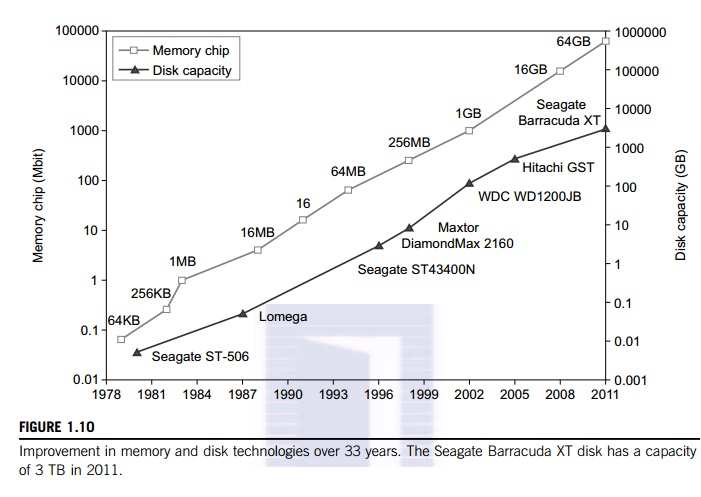
1.2.3.1 Memory Technology
The upper curve in Figure
1.10 plots the growth of DRAM chip capacity from 16 KB in 1976 to 64 GB in
2011. This shows that memory chips have experienced a 4x increase in capacity
every three years. Memory access time did not improve much in the past. In
fact, the memory wall problem is getting worse as the processor gets faster.
For hard drives, capacity increased from 260 MB in 1981 to 250 GB in 2004. The
Seagate Barracuda XT hard drive reached 3 TB in 2011. This represents an
approximately 10x increase in capacity every eight years. The capacity increase
of disk arrays will be even greater in the years to come. Faster processor
speed and larger memory capacity result in a wider gap between processors and memory.
The memory wall may become even worse a problem limiting the CPU perfor-mance
in the future.
3.2
Disks and Storage Technology
Beyond 2011, disks or disk
arrays have exceeded 3 TB in capacity. The lower curve in Figure 1.10 shows the
disk storage growth in 7 orders of magnitude in 33 years. The rapid growth of
flash memory and solid-state
drives (SSDs) also impacts the future of HPC and HTC systems. The
mor-tality rate of SSD is not bad at all. A typical SSD can handle 300,000 to 1
million write cycles per
block. So the SSD can last
for several years, even under conditions of heavy write usage. Flash and SSD
will demonstrate impressive speedups in many applications.
Eventually,
power consumption, cooling, and packaging will limit large system development.
Power increases linearly with respect to clock frequency and quadratic ally
with respect to voltage applied on chips. Clock rate cannot be increased
indefinitely. Lowered voltage supplies are very much in demand. Jim Gray once
said in an invited talk at the University of Southern California,
“Tape units are dead, disks are tape units,
flashes are disks, and memory are caches now.” This clearly paints the future for disk and storage
technology. In 2011, the SSDs are still too expensive to replace stable disk
arrays in the storage market.
3.3
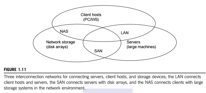
System-Area Interconnects
The nodes in small clusters
are mostly interconnected by an Ethernet switch or a local area network (LAN). As Figure 1.11 shows,
a LAN typically is used to connect client hosts to big servers. A storage area network (SAN) connects servers to
network storage such as disk arrays. Network attached storage (NAS) connects client hosts directly to the
disk arrays. All three types of networks often appear in a large cluster built with
commercial network components. If no large distributed storage is shared, a
small cluster could be built with a multiport Gigabit Ethernet switch plus
copper cables to link the end machines. All three types of networks are
commercially available.
3.4
Wide-Area Networking
The lower curve in Figure
1.10 plots the rapid growth of Ethernet bandwidth from 10 Mbps in 1979 to 1
Gbps in 1999, and 40 ~ 100 GE in 2011. It has been speculated that 1 Tbps
network links will become available by 2013. According to Berman, Fox, and Hey
[6], network links with 1,000, 1,000, 100, 10, and 1 Gbps bandwidths were
reported, respectively, for international, national, organization, optical
desktop, and copper desktop connections in 2006.
An
increase factor of two per year on network performance was reported, which is
faster than Moore’s law on CPU speed doubling
every 18 months. The implication is that more computers will be used
concurrently in the future. High-bandwidth networking increases the capability
of building massively distributed systems. The IDC 2010 report predicted that
both InfiniBand and Ethernet will be the two major interconnect choices in the
HPC arena. Most data centers are using Gigabit Ethernet as the interconnect in
their server clusters.
4. Virtual Machines and Virtualization
Middleware
A conventional computer has a
single OS image. This offers a rigid architecture that tightly couples
application software to a specific hardware platform. Some software running
well on one machine may not be executable on another platform with a different
instruction set under a fixed OS. Virtual machines (VMs) offer novel solutions to underutilized
resources, application inflexibility, software manageability, and security concerns in
existing physical machines.
Today, to build large
clusters, grids, and clouds, we need to access large amounts of computing,
storage, and networking resources in a virtualized manner. We need to aggregate
those resources, and hopefully, offer a single system image. In particular, a
cloud of provisioned resources must rely on virtualization of processors,
memory, and I/O facilities dynamically. We will cover virtualization in Chapter
3. However, the basic concepts of virtualized resources, such as VMs, virtual
storage, and virtual networking and their virtualization software or
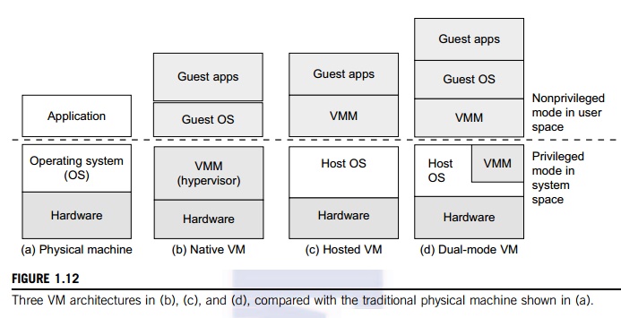
middleware, need to be introduced first. Figure 1.12 illustrates the
architectures of three VM configurations.
4.1
Virtual Machines
In Figure 1.12, the host machine
is equipped with the physical hardware, as shown at the bottom of the figure.
An example is an x-86 architecture desktop running its installed Windows OS, as
shown in part (a) of the figure. The VM can be provisioned for any hardware
system. The VM is built with virtual resources managed by a guest OS to run a
specific application. Between the VMs and the host platform, one needs to
deploy a middleware layer called a virtual machine monitor (VMM). Figure 1.12(b) shows a
native VM installed with the use of a VMM called a hypervisor in privi-leged mode. For example, the hardware
has x-86 architecture running the Windows system.
The
guest OS could be a Linux system and the hypervisor is the XEN system developed
at Cambridge University. This hypervisor approach is also called bare-metal VM, because the hypervi-sor handles the bare
hardware (CPU, memory, and I/O) directly. Another architecture is the host VM
shown in Figure 1.12(c). Here the VMM runs in nonprivileged mode. The host OS
need not be modi-fied. The VM can also be implemented with a dual mode, as
shown in Figure 1.12(d). Part of the VMM runs at the user level and another
part runs at the supervisor level. In this case, the host OS may have to be
modified to some extent. Multiple VMs can be ported to a given hardware system
to support the virtualization process. The VM approach offers hardware
independence of the OS and applications. The user application running on its
dedicated OS could be bundled together as a virtual appliance that can be ported to any hardware platform.
The VM could run on an OS different from that of the host computer.
4.2
VM Primitive Operations
The VMM provides the VM
abstraction to the guest OS. With full virtualization, the VMM exports a VM
abstraction identical to the physical machine so that a standard OS such as
Windows 2000 or Linux can run just as it would on the physical hardware.
Low-level VMM operations are indicated by Mendel Rosenblum [41] and illustrated
in Figure 1.13.
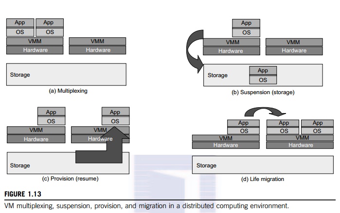
• First, the VMs can be
multiplexed between hardware machines, as shown in Figure 1.13(a).
• Second, a VM can be suspended
and stored in stable storage, as shown in Figure 1.13(b).
• Third, a suspended VM can be
resumed or provisioned to a new hardware platform, as shown in Figure 1.13(c).
•
Finally, a VM can be migrated from one hardware
platform to another, as shown in Figure 1.13(d).
These VM
operations enable a VM to be provisioned to any available hardware platform.
They also enable flexibility in porting distributed application executions. Furthermore,
the VM approach will significantly enhance the utilization of server resources.
Multiple server functions can be consolidated on the same hardware platform to
achieve higher system efficiency. This will eliminate server sprawl via
deployment of systems as VMs, which move transparency to the shared hardware.
With this approach, VMware claimed that server utilization could be increased
from its current 5–15 percent to 60–80 percent.
4.3
Virtual Infrastructures
Physical resources for
compute, storage, and networking at the bottom of Figure 1.14 are mapped to the
needy applications embedded in various VMs at the top. Hardware and software
are then sepa-rated. Virtual infrastructure is what connects resources to
distributed applications. It is a dynamic mapping of system resources to
specific applications. The result is decreased costs and increased efficiency
and responsiveness. Virtualization for server consolidation and containment is
a good example of this. We will discuss VMs and virtualization support in
Chapter 3. Virtualization support for clusters, clouds, and grids is covered in
Chapters 3, 4, and 7, respectively.
5. Data Center Virtualization for
Cloud Computing
In this
section, we discuss basic architecture and design considerations of data
centers. Cloud architecture is built with commodity hardware and network
devices. Almost all cloud platforms choose the popular x86 processors. Low-cost
terabyte disks and Gigabit Ethernet are used to build data centers. Data center
design emphasizes the performance/price ratio over speed performance alone. In
other words, storage and energy efficiency are more important than shear speed
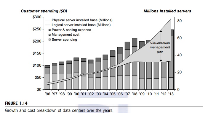
performance. Figure 1.13 shows the server growth and cost breakdown of data
centers over the past 15 years. Worldwide, about 43 million servers are in use
as of 2010. The cost of utilities exceeds the cost of hardware after three
years.
5.1
Data Center Growth and Cost Breakdown
A large data center may be
built with thousands of servers. Smaller data centers are typically built with
hundreds of servers. The cost to build and maintain data center servers has
increased over the years. According to a 2009 IDC report (see Figure 1.14),
typically only 30 percent of data center costs goes toward purchasing IT
equipment (such as servers and disks), 33 percent is attributed to the chiller,
18 percent to the uninterruptible
power supply (UPS), 9 percent to computer
room air conditioning
(CRAC), and the remaining 7 percent to power distribution, lighting, and
transformer costs. Thus, about 60 percent
of the cost to run a data center is allocated to management and main-tenance.
The server purchase cost did not increase much with time. The cost of
electricity and cool-ing did increase from 5 percent to 14 percent in 15 years.
5.2
Low-Cost Design Philosophy
High-end switches or routers
may be too cost-prohibitive for building data centers. Thus, using
high-bandwidth networks may not fit the economics of cloud computing. Given a
fixed budget, commodity switches and networks are more desirable in data
centers. Similarly, using commodity x86 servers is more desired over expensive
mainframes. The software layer handles network traffic balancing, fault
tolerance, and expandability. Currently, nearly all cloud computing data
centers use Ethernet as their fundamental network technology.
5.3
Convergence of Technologies
Essentially, cloud computing
is enabled by the convergence of technologies in four areas: (1) hard-ware
virtualization and multi-core chips, (2) utility and grid computing, (3) SOA,
Web 2.0, and WS mashups, and (4) atonomic computing and data center automation.
Hardware virtualization and mul-ticore chips enable the existence of dynamic
configurations in the cloud. Utility and grid computing technologies lay the
necessary foundation for computing clouds. Recent advances in SOA, Web 2.0, and
mashups of platforms are pushing the cloud another step forward. Finally,
achievements in autonomic computing and automated data center operations
contribute to the rise of cloud computing.
Jim Gray
once posted the following question: “Science faces a data deluge. How to manage and analyze information?” This implies that science and
our society face the same challenge of data deluge. Data comes from sensors, lab
experiments, simulations, individual archives, and the web in all scales and
formats. Preservation, movement, and access of massive data sets require
generic tools supporting high-performance, scalable file systems, databases,
algorithms, workflows, and visualization. With science becoming data-centric, a
new paradigm of scientific discovery is becom-ing based on data-intensive
technologies.
On
January 11, 2007, the Computer
Science and Telecommunication Board (CSTB) recom-mended fostering tools for data capture,
data creation, and data analysis. A cycle of interaction exists among four
technical areas. First, cloud technology is driven by a surge of interest in
data deluge. Also, cloud computing impacts e-science greatly, which explores
multicore and parallel computing technologies. These two hot areas enable the
buildup of data deluge. To support data-intensive computing, one needs to
address workflows, databases, algorithms, and virtualization issues.
By
linking computer science and technologies with scientists, a spectrum of
e-science or e-research applications in biology, chemistry, physics, the social
sciences, and the humanities has generated new insights from interdisciplinary
activities. Cloud computing is a transformative approach as it promises much
more than a data center model. It fundamentally changes how we interact with
information. The cloud provides services on demand at the infrastructure,
platform, or software level. At the platform level, MapReduce offers a new
programming model that transpar-ently handles data parallelism with natural
fault tolerance capability. We will discuss MapReduce in more detail in Chapter
6.
Iterative MapReduce extends
MapReduce to support a broader range of data mining algorithms commonly used in
scientific applications. The cloud runs on an extremely large cluster of
commod-ity computers. Internal to each cluster node, multithreading is
practiced with a large number of cores in many-core GPU clusters.
Data-intensive science, cloud computing, and multicore comput-ing are
converging and revolutionizing the next generation of computing in
architectural design and programming challenges. They enable the pipeline: Data
becomes information and knowledge, and in turn becomes machine wisdom as
desired in SOA.
Related Topics