Subband Coding

Subband Coding:

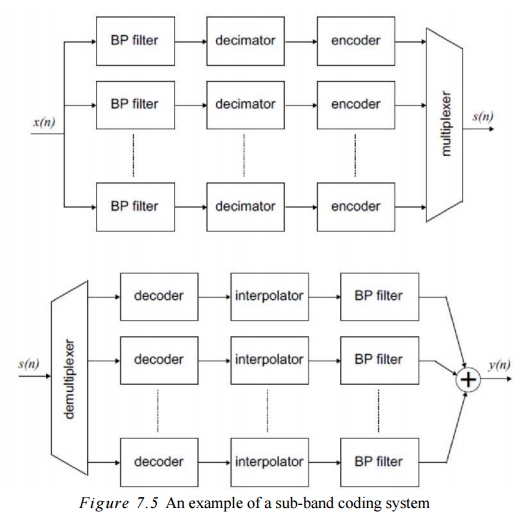
Another coding method is sub-band coding (SBC) (see Figure 7.5) which belongs to the class of waveform coding methods, in which the frequency domain properties of the input signal arc utilized to achieve data compression.

The basic idea is that the input speech signal is split into sub-bands using band-pass filters. The sub-band signals arc then encoded using ADPCM or other techniques. In this way, the available data transmission capacity can be allocated between bands according to pcrccptual criteria, enhancing the speech quality as pcrceivcd by listeners. A sub-band that is more ‘important’ from the human listening point of view can be allocated more bits in the data stream, while less important sub-bands will use fewer bits.

A typical setup for a sub-band codcr would be a bank of N(digital) bandpass filters followed by dccimators, encoders (for instance ADPCM) and a multiplexer combining the data bits coming from the sub-band channels. The output of the multiplexer is then transmitted to the sub-band dccodcr having a demultiplexer splitting the multiplexed data stream back into Nsub-band channels. Every sub-band channel has a dccodcr (for instance ADPCM), followed by an interpolator and a band-pass filter. Finally, the outputs of the band-pass filters are summed and a reconstructed output signal results.

Sub-band coding is commonly used at bit rates between 9.6 kbits/s and 32 kbits/s and performs quite well. The complexity of the system may however be considerable if the number of sub-bands is large. The design of the band-pass filters is also a critical topic when working with sub-band coding systems.

Vocoders and LPC

In the methods described above (APC, SBC and ADPCM), speech signal applications have been used as examples. By modifying the structure and parameters of the predictors and filters, the algorithms may also be used for other signal types. The main objective was to achieve a reproduction that was as faithful as possible to the original signal. Data compression was possible by removing redundancy in the time or frequency domain.

The class of vocoders (also called source coders) is a special class of data compression devices aimed only at spcech signals. The input signal is analysed and described in terms of speech model parameters. These parameters are then used to synthesize a voice pattern having an acceptable level of perceptual quality. Hence, waveform accuracy is not the main goal, as in the previous methods discussed.

The first vocoder was designed by H. Dudley in the 1930s and demonstrated at the ‘New York Fair’ in 1939* Vocoders have become popular as they achieve reasonably good speech quality at low data rates, from 2A kbits/s to 9,6 kbits/s. There arc many types of vocoders (Marvcn and Ewers, 1993), some of the most common techniques will be briefly presented below.

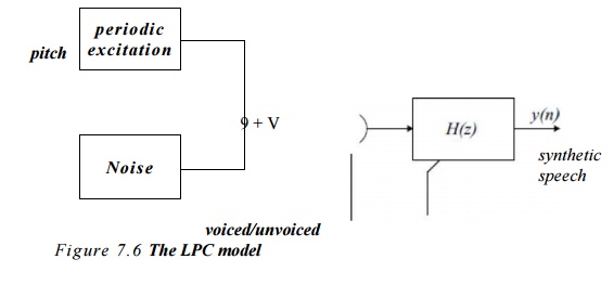
Most vocoders rely on a few basic principles. Firstly, the characteristics of the spccch signal is assumed to be fairly constant over a time of approximately 20 ms, hcncc most signal processing is performed on (overlapping) data blocks of 20 40 ms length. Secondly, the spccch model consists of a time varying filter corresponding to the acoustic properties of the mouth and an excitation signal. The cxeilalion signal is cither a periodic waveform, as crcatcd by the vocal chords, or a random noise signal for production of ‘unvoiced' sounds, for example ‘s’ and T. The filter parameters and excitation parameters arc assumed to be independent of each other and are commonly coded separately.

Linear predictive coding (LPC) is a popular method, which has however been replaced by newer approaches in many applications. LPC works exceed-ingly well at low bit rates and the LPC parameters contain sufficient information of the spccch signal to be used in spccch recognition applications. The LPC model is shown in Figure 7*6.

LPC is basically an autn-regressive model (sec Chapter 5) and the vocal tract is modelled as a time-varying all-pole filter (HR filter) having the transfer function H(z)

The output sample at time n is a linear combination of p previous samples and the excitation signal (linear predictive coding). The filter coefficients a_k arc time varying.

The model above describes how to synthesize the speech given the pitch information (if noise or pet iodic excitation should be used), the gain and the filter parameters. These parameters must be determined by the cncoder or the analyser, taking the original spccch signal x(n) as input.

The analyser windows the spccch signal in blocks of 20-40 ms. usually with a Hamming window (see Chapter 5). These blocks or ‘frames’ arc repeated every 10—30 ms, hence there is a certain overlap in time. Every frame is then analysed with respect to the parameters mentioned above.

Firstly, the pitch frequency is determined. This also tells whether we arc dealing with a voiced or unvoiccd spccch signal. This is a crucial part of the system and many pitch detection algorithms have been proposed. If the segment of the spccch signal is voiced and has a dear periodicity or if it is unvoiced and not pet iodic, things arc quite easy* Segments having properties in between these two extremes are difficult to analyse. No algorithm has been found so far that is ¹perfect* for all listeners.

Now, the second step of the analyser is to determine the gain and the filter parameters. This is done by estimating the spccch signal using an adaptive predictor. The predictor has the same structure and order as the filter in the synthesizer, Hencc, the output of the predictor is

- i(n) — - tf]jt(/7— 1) — a ₂ x(n — 2) — ... — OpX(n—p)     (7-19)

where i(rt) is the predicted input spcech signal and jc(rt) is the actual input signal. The filter coefficients a_k are determined by minimizing the square error

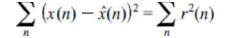
This can be done in different ways, cither by calculating the auto-corrc- lation coefficients and solving the Yule Walker equations (see Chapter 5) or by using some recursive, adaptive filter approach (see Chapter 3),

So, for every frame, all the parameters above arc determined and irans - mittcd to the synthesiser, where a synthetic copy of the spccch is generated.

An improved version of LPC is residual excited linear prediction (RELP).

Let us take a closer look at the error or residual signal r(fi) resulting from the prediction in the analyser (equation (7.19)). The residual signal (wc arc try ing to minimize) can be expressed as

r(n)= *(«) -i(rt)

= jf(rt) + a^x(n— 1) + a₂ x(n — 2) -h *.. + a_p x(ft—p) <7-21) From this it is straightforward to find out that the corresponding expression using the z-transforms is

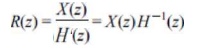
Hence, the prcdictor can be regarded as an ‘inverse’ filter to the LPC model filter. If we now pass this residual signal to the synthesizer and use it to excite the LPC filter, that is E(z) - R(z), instead of using the noise or periodic waveform sources we get

Y(z) = E(z)H(z) = R(z)H(z) = X(z)H~\z)H(z) = X(z) (7.23)

In the ideal case, we would hence get the original speech signal back. When minimizing the variance of the residual signal (equation (7.20)), we gathered as much information about the spccch signal as possible using this model in the filter coefficients a_k . The residual signal contains the remaining information. If the model is well suited for the signal type (speech signal), the residual signal is close to white noise, having a flat spectrum. In such a case we can get away with coding only a small range of frequencies, for instance 0-1 kHz of the residual signal. At the synthesizer, this baseband is then repeated to generate higher frequencies. This signal is used to excite the LPC filter

Vocoders using RELP are used with transmission rates of 9.6 kbits/s. The advantage of RELP is a better speech quality compared to LPC for the same bit rate. However, the implementation is more computationally demanding.

Another possible extension of the original LPC approach is to use multipulse excited linear predictive coding (MLPC). This extension is an attempt to make the synthesized spcech less ‘mechanical’, by using a number of different pitches of the excitation pulses rather than only the two (periodic and noise) used by standard LPC.

The MLPC algorithm sequentially detects k pitches in a speech signal. As soon as one pitch is found it is subtracted from the signal and detection starts over again, looking for the next pitch. Pitch information detection is a hard task and the complexity of the required algorithms is often considerable. MLPC however offers a better spcech quality than LPC for a given bit rate and is used in systems working with 4.S-9.6 kbits/s.

Yet another extension of LPC is the code excited linear prediction (CELP).

The main feature of the CELP compared to LPC is the way in which the filter coefficients are handled. Assume that we have a standard LPC system, with a filter of the order p . If every coefficient a_k requires N bits, we need to transmit N-p bits per frame for the filter parameters only. This approach is all right if all combinations of filter coefficients arc equally probable. This is however not the case. Some combinations of coefficients are very probable, while others may never occur. In CELP, the coefficient combinations arc represented by p dimensional vectors. Using vector quantization techniques, the most probable vectors are determined. Each of these vectors are assigned an index and stored in a codebook. Both the analyser and synthesizer of course have identical copies of the codebook, typically containing 256-512 vectors. Hcncc, instead of transmitting N-p bits per frame for the filter parameters only 8-9 bits arc needed.

This method offers high-quality spcech at low-bit rates but requires consid-erable computing power to be able to store and match the incoming spcech to the ‘standard’ sounds stored in the codebook. This is of course especially true if the codebook is large. Speech quality degrades as the codebook size decreases.

Most CELP systems do not perform well with respect to higher frequency components of the spccch signal at low hit rates. This is countcractcd in

There is also a variant of CELP called vector sum excited linear prediction (VSELP). The main difference between CELP and VSELP is the way the codebook is organized. Further, since VSELP uses fixed point arithmetic algorithms, it is possible to implement using cheaper DSP chips than Adaptive Filters

The signal degradation in some physical systems is time varying, unknown, or possibly both. For example,consider a high-speed modem for transmitting and receiving data over telephone channels. It employs a filter called a channel equalizer to compensate for the channel distortion. Since the dial-up communication channels have different and time-varying characteristics on each connection, the equalizer must be an adaptive filter.