Adaptive Filter

Adaptive Filter:

Adaptive filters modify their characteristics to achieve certain objectives by automatically updating their coefficients. Many adaptive filter structures and adaptation algorithms have been developed for different applications. This chapter presents the most widely used adaptive filters based on the FIR filter with the least-mean -square (LMS) algorithm. These adaptive filters are relatively simple to design and implement. They are well understood with regard to stability, convergence speed, steady-state performance, and finite-precision effects.

Introduction to Adaptive Filtering

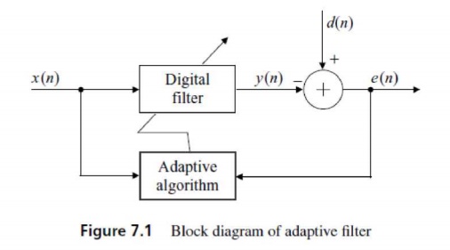
An adaptive filter consists of two distinct parts - a digital filter to perform the desired filtering, and an adaptive algorithm to adjust the coefficients (or weights) of the filter. A general form of adaptive filter is illustrated in Figure 7.1, where d(n) is a desired (or primary input) signal, y(n) is the output of a digital filter driven by a reference input signal x(n), and an error signal e(n) is the difference between d(n) and y(n). The adaptive algorithm adjusts the filter coefficients to minimize the mean-square value of e(n). Therefore, the filter weights are updated so that the error is progressively minimized on a sample-bysample basis.

In general, there are two types of digital filters that can be used for adaptive filtering: FIR and IIR filters. The FIR filter is always stable and can provide a linear-phase response. On the other hand, the IIR

filter involves both zeros and poles. Unless they are properly controlled, the poles in the filter may move outside the unit circle and result in an unstable system during the adaptation of coefficients. Thus, the adaptive FIR filter is widely used for practical real-time applications. This chapter focuses on the class of adaptive FIR filters.

The most widely used adaptive FIR filter is depicted in Figure 7.2. The filter output signal is computed

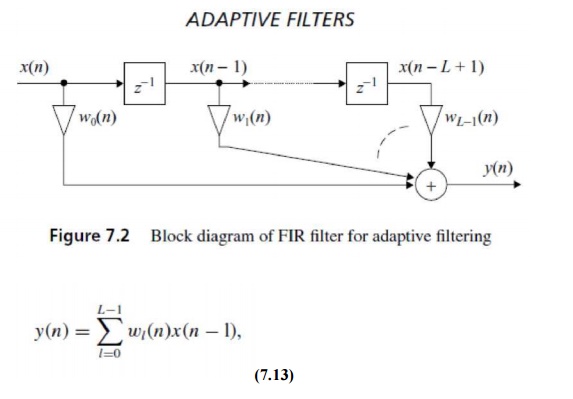
, where the filter coefficients wl (n) are time varying and updated by the adaptive algorithms that will be discussed next.

We define the input vector at time n as

x(n) = [x(n)x(n - 1) . . . x(n - L + 1)]T , (7.14) and the weight vector at time n as

w(n) = [w0(n)w1(n) . . . wL-1(n)]T . (7.15) Equation (7.13) can be expressed in vector form as y(n) = wT (n)x(n) = xT (n)w(n). (7.16)

The filter outputy(n) is compared with the desired d(n) to obtain the error signal e(n) = d(n) - y(n) = d(n) - wT (n)x(n). (7.17)

Our objective is to determine the weight vector w(n) to minimize the predetermined performance (or cost) function.

Performance Function:

The adaptive filter shown in Figure 7.1 updates the coefficients of the digital filter to optimize some predetermined performance criterion. The most commonly used performance function is based on the mean-square error (MSE).