Properties of Relational Decompositions

Properties of Relational Decompositions

We now turn our attention to the process of decomposition that we used through-out Chapter 15 to decompose relations in order to get rid of unwanted dependencies and achieve higher normal forms. In Section 16.2.1 we give examples to show that looking at an individual relation to test whether it is in a higher normal form does not, on its own, guarantee a good design; rather, a set of relations that together form the relational database schema must possess certain additional properties to ensure a good design. In Sections 16.2.2 and 16.2.3 we discuss two of these proper-ties: the dependency preservation property and the nonadditive (or lossless) join property. Section 16.2.4 discusses binary decompositions and Section 16.2.5 dis-cusses successive nonadditive join decompositions.

1. Relation Decomposition and Insufficiency of Normal Forms

The relational database design algorithms that we present in Section 16.3 start from a single universal relation schema R = {A₁, A₂, ..., A_n} that includes all the attributes of the database. We implicitly make the universal relation assumption, which states that every attribute name is unique. The set F of functional dependencies that should hold on the attributes of R is specified by the database designers and is made available to the design algorithms. Using the functional dependencies, the algorithms decompose the universal relation schema R into a set of relation schemas D = {R₁, R₂, ..., R_m} that will become the relational database schema; D is called a decomposition of R.

We must make sure that each attribute in R will appear in at least one relation schema R_i in the decomposition so that no attributes are lost; formally, we have

This is called the attribute preservation condition of a decomposition.

Another goal is to have each individual relation R_i in the decomposition D be in BCNF or 3NF. However, this condition is not sufficient to guarantee a good data-base design on its own. We must consider the decomposition of the universal rela-tion as a whole, in addition to looking at the individual relations. To illustrate this point, consider the EMP_LOCS(Ename, Plocation) relation in Figure 15.5, which is in 3NF and also in BCNF. In fact, any relation schema with only two attributes is auto-matically in BCNF.⁵ Although EMP_LOCS is in BCNF, it still gives rise to spurious tuples when joined with EMP_PROJ (Ssn, Pnumber, Hours, Pname, Plocation), which is not in BCNF (see the result of the natural join in Figure 15.6). Hence, EMP_LOCS represents a particularly bad relation schema because of its convoluted semantics by which Plocation gives the location of one of the projects on which an employee works. Joining EMP_LOCS with PROJECT(Pname, Pnumber, Plocation, Dnum) in Figure 15.2—which is in BCNF—using Plocation as a joining attribute also gives rise to spurious tuples. This underscores the need for other criteria that, together with the conditions of 3NF or BCNF, prevent such bad designs. In the next three subsections we discuss such additional conditions that should hold on a decomposition D as a whole.

2. Dependency Preservation Property of a Decomposition

It would be useful if each functional dependency X→Y specified in F either appeared directly in one of the relation schemas R_i in the decomposition D or could be inferred from the dependencies that appear in some R_i. Informally, this is the dependency preservation condition. We want to preserve the dependencies because each dependency in F represents a constraint on the database. If one of the depen-dencies is not represented in some individual relation R_i of the decomposition, we cannot enforce this constraint by dealing with an individual relation. We may have to join multiple relations so as to include all attributes involved in that dependency.

It is not necessary that the exact dependencies specified in F appear themselves in individual relations of the decomposition D. It is sufficient that the union of the dependencies that hold on the individual relations in D be equivalent to F. We now define these concepts more formally.

Definition. Given a set of dependencies F on R, the projection of F on R_i, denoted by π_Ri(F) where R_i is a subset of R, is the set of dependencies X → Y in F⁺ such that the attributes in X ∪ Y are all contained in R_i. Hence, the projection of F on each relation schema R_i in the decomposition D is the set of functional dependencies in F⁺, the closure of F, such that all their left- and right-hand-side attributes are in R_i. We say that a decomposition D = {R₁, R₂, ..., R_m} of R is dependency-preserving with respect to F if the union of the

projections of F on each Ri  in D is equivalent to F; that is, ((π_R (F)) ∪ ... ∪1

(π_Rm(F)))⁺ = F⁺.

If a decomposition is not dependency-preserving, some dependency is lost in the decomposition. To check that a lost dependency holds, we must take the JOIN of two or more relations in the decomposition to get a relation that includes all left-and right-hand-side attributes of the lost dependency, and then check that the dependency holds on the result of the JOIN—an option that is not practical.

An example of a decomposition that does not preserve dependencies is shown in Figure 15.13(a), in which the functional dependency FD2 is lost when LOTS1A is decomposed into {LOTS1AX, LOTS1AY}. The decompositions in Figure 15.12, how-ever, are dependency-preserving. Similarly, for the example in Figure 15.14, no mat-ter what decomposition is chosen for the relation TEACH(Student, Course, Instructor) from the three provided in the text, one or both of the dependencies originally present are bound to be lost. We state a claim below related to this property without providing any proof.

Claim 1. It is always possible to find a dependency-preserving decomposition D with respect to F such that each relation R_i in D is in 3NF.

In Section 16.3.1, we describe Algorithm 16.4, which creates a dependency-preserving decomposition D = {R₁, R₂, ..., R_m} of a universal relation R based on a set of functional dependencies F, such that each R_i in D is in 3NF.

3. Nonadditive (Lossless) Join Property of a Decomposition

Another property that a decomposition D should possess is the nonadditive join property, which ensures that no spurious tuples are generated when a NATURAL JOIN operation is applied to the relations resulting from the decomposition. We already illustrated this problem in Section 15.1.4 with the example in Figures 15.5 and 15.6. Because this is a property of a decomposition of relation schemas, the condition of no spurious tuples should hold on every legal relation state—that is, every relation state that satisfies the functional dependencies in F. Hence, the lossless join property is always defined with respect to a specific set F of dependencies.

Definition. Formally, a decomposition D = {R₁, R₂, ..., R_m} of R has the lossless (nonadditive) join property with respect to the set of dependencies F on R if, for every relation state r of R that satisfies F, the following holds, where _* is the NATURAL JOIN of all the relations in D: _*(π_R1(r), ..., π_Rm(r)) = r.

The word loss in lossless refers to loss of information, not to loss of tuples. If a decom-position does not have the lossless join property, we may get additional spurious tuples after the PROJECT (π) and NATURAL JOIN (*) operations are applied; these additional tuples represent erroneous or invalid information. We prefer the term nonadditive join because it describes the situation more accurately. Although the term lossless join has been popular in the literature, we will henceforth use the term nonadditive join, which is self-explanatory and unambiguous. The nonadditive join property ensures that no spurious tuples result after the application of PROJECT and JOIN operations. We may, however, sometimes use the term lossy design to refer to a design that represents a loss of information (see example at the end of Algorithm 16.4).

The decomposition of EMP_PROJ(Ssn, Pnumber, Hours, Ename, Pname, Plocation) in Figure 15.3 into EMP_LOCS(Ename, Plocation) and EMP_PROJ1(Ssn, Pnumber, Hours,

Pname, Plocation) in Figure 15.5 obviously does not have the nonadditive join property, as illustrated by Figure 15.6. We will use a general procedure for testing whether any decomposition D of a relation into n relations is nonadditive with respect to a set of given functional dependencies F in the relation; it is presented as Algorithm 16.3 below. It is possible to apply a simpler test to check if the decomposition is nonaddi-tive for binary decompositions; that test is described in Section 16.2.4.

Algorithm 16.3. Testing for Nonadditive Join Property

Input: A universal relation R, a decomposition D = {R₁, R₂, ..., R_m} of R, and a set F of functional dependencies.

Note: Explanatory comments are given at the end of some of the steps. They fol-low the format: (* comment *).

        Create an initial matrix S with one row i for each relation R_i in D, and one column j for each attribute A_j in R.

        Set S(i, j):= b_ij for all matrix entries. (* each b_ij is a distinct symbol associated with indices (i, j) *).

        For each row i representing relation schema R_i {for each column j representing attribute A_j

        {if (relation R_i includes attribute A_j) then set S(i, j):= a_j ;};}; (* each a_j is a distinct symbol associated with index ( j) *).

        Repeat the following loop until a complete loop execution results in no

changes to S

{for each functional dependency X → Y in F

{for all rows in S that have the same symbols in the columns corresponding to attributes in X

{make the symbols in each column that correspond to an attribute in Y be the same in all these rows as follows: If any of the rows has an a sym-bol for the column, set the other rows to that same a symbol in the col-umn. If no a symbol exists for the attribute in any of the rows, choose one of the b symbols that appears in one of the rows for the attribute and set the other rows to that same b symbol in the column ;} ; } ;};

        If a row is made up entirely of a symbols, then the decomposition has the nonadditive join property; otherwise, it does not.

Given a relation R that is decomposed into a number of relations R₁, R₂, ..., R_m, Algorithm 16.3 begins the matrix S that we consider to be some relation state r of R. Row i in S represents a tuple t_i (corresponding to relation R_i) that has a symbols in the columns that correspond to the attributes of R_i and b symbols in the remaining columns. The algorithm then transforms the rows of this matrix (during the loop in step 4) so that they represent tuples that satisfy all the functional dependencies in F. At the end of step 4, any two rows in S—which represent two tuples in r—that agree in their values for the left-hand-side attributes X of a functional dependency X → Y in F will also agree in their values for the right-hand-side attributes Y. It can be shown that after applying the loop of step 4, if any row in S ends up with all a sym-bols, then the decomposition D has the nonadditive join property with respect to F.

If, on the other hand, no row ends up being all a symbols, D does not satisfy the lossless join property. In this case, the relation state r represented by S at the end of the algorithm will be an example of a relation state r of R that satisfies the depend-encies in F but does not satisfy the nonadditive join condition. Thus, this relation serves as a counterexample that proves that D does not have the nonadditive join property with respect to F. Note that the a and b symbols have no special meaning at the end of the algorithm.

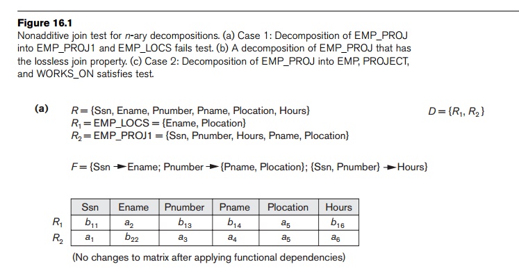
Figure 16.1(a) shows how we apply Algorithm 16.3 to the decomposition of the EMP_PROJ relation schema from Figure 15.3(b) into the two relation schemas EMP_PROJ1 and EMP_LOCS in Figure 15.5(a). The loop in step 4 of the algorithm cannot change any b symbols to a symbols; hence, the resulting matrix S does not have a row with all a symbols, and so the decomposition does not have the non-additive join property.

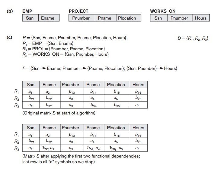
Figure 16.1(b) shows another decomposition of EMP_PROJ (into EMP, PROJECT, and WORKS_ON) that does have the nonadditive join property, and Figure 16.1(c) shows how we apply the algorithm to that decomposition. Once a row consists only of a symbols, we conclude that the decomposition has the nonadditive join property, and we can stop applying the functional dependencies (step 4 in the algorithm) to the matrix S.

Figure 16.1

Nonadditive join test for n-ary decompositions. (a) Case 1: Decomposition of EMP_PROJ into EMP_PROJ1 and EMP_LOCS fails test. (b) A decomposition of EMP_PROJ that has the lossless join property. (c) Case 2: Decomposition of EMP_PROJ into EMP, PROJECT, and WORKS_ON satisfies test.

4. Testing Binary Decompositions for the Nonadditive Join Property

Algorithm 16.3 allows us to test whether a particular decomposition D into n relations obeys the nonadditive join property with respect to a set of functional dependencies F. There is a special case of a decomposition called a binary decomposition—decomposition of a relation R into two relations. We give an easier test to apply than Algorithm 16.3, but while it is very handy to use, it is limited to binary decompositions only.

Property NJB (Nonadditive Join Test for Binary Decompositions). A decomposition D = {R₁, R₂} of R has the lossless (nonadditive) join property with respect to a set of functional dependencies F on R if and only if either

        The FD ((R₁ ∩ R₂) → (R₁ – R₂)) is in F⁺, or

        The FD ((R₁ ∩ R₂) → (R₂ – R₁)) is in F⁺

You should verify that this property holds with respect to our informal successive normalization examples in Sections 15.3 and 15.4. In Section 15.5 we decomposed LOTS1A into two BCNF relations LOTS1AX and LOTS1AY, and decomposed the TEACH relation in Figure 15.14 into the two relations {Instructor, Course} and {Instructor, Student}. These are valid decompositions because they are nonadditive per the above test.

5. Successive Nonadditive Join Decompositions

We saw the successive decomposition of relations during the process of second and third normalization in Sections 15.3 and 15.4. To verify that these decompositions are nonadditive, we need to ensure another property, as set forth in Claim 2.

Claim 2 (Preservation of Nonadditivity in Successive Decompositions). If a decomposition D = {R₁, R₂, ..., R_m} of R has the nonadditive (lossless) join property with respect to a set of functional dependencies F on R, and if a decomposition D_i = {Q₁, Q₂, ..., Q_k} of R_i has the nonadditive join property with respect to the projection of F on R_i, then the decomposition D₂ = {R₁, R₂, ..., R_i−1, Q₁, Q₂, ..., Q_k, R_i+1, ..., R_m} of R has the nonadditive join property with respect to F.