Production Concepts and Mathematical Models

PRODUCTION CONCEPTS AND MATHEMATICAL MODELS

A number of production concepts are quantitative, or they require a quantitative approach to measure them. The purpose of this section is to define some of these concepts. In subsequent chapters, we refer back to these production concepts in our discussion of specific topics in automation and production systems. The models developed in this section are ideal, in the sense that they neglect some of the realities and complications that are present in the factory. For example, our models do not include the effect of scrap rates. In some manufacturing operations, the percentage of scrap produced is high enough to adversely affect production rate, plant capacity, and product costs. Most of these issues are considered in later chapters as we focus on specific types of production systems.

1     Production Rate

The production rate for an individual processing or assembly operation is usually expressed as an hourly rate, that is, parts or products per hour. Let us consider how this rate is determined for the three types of production: job shop production, batch production, and mass production.

For any production operation, the operation cycle time T_c is defined as the time that one work unit spends being processed or assembled. It is the time between when one work unit begins processing (or assembly) and when the next unit begins. T_c is the time an individual part spends at the machine, but not all of this time is productive (recall the Merchant study, Section 2.2.2). In a typical processing operation, such as machining, T_c consists of: (1) actual machining operation time, (2) workpart handling time, and (3) tool handling time per workpiece. As an equation, this can be expressed:

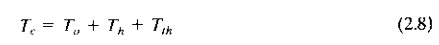
where T_c=operation cycle time (min pc), T_o=time of the actual processing or assembly operation (min pc), T_h=handling time (min pc), and T_th=tool handling time (min pc). The tool handling time consists of time spent changing tools when they wear out, time changing from one tool to the next, tool indexing time for indexable inserts or for tools on a turret lathe or turret drill, tool repositioning for a next pass, and so on. Some of these tool handling activities do not occur every cycle; therefore, they must be spread over the number of parts between their occurrences to obtain an average time per workpiece.

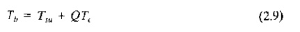
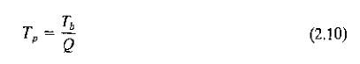
where T_b=batch processing time (min), T_su=setup time to prepare for the batch( min), Q=batch quantity (pc), and T_c=operation cycle time per work unit (min cycle). We assume that one work unit is completed each cycle and so T_c also has units of min pc. If more than one part is produced each cycle, then Eq. (2.9) must be adjusted accordingly. Dividing batch time by batch quantity, we have the average production time per work unit T_p for the given machine:

The average production rate for the machine is simply the reciprocal of production time. It is usually expressed as an hourly rate:

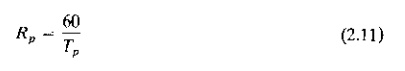
where R_p=hourly production rate (pc hr), T_p=average production time per minute (min pc), and the constant 60 converts minutes to hours.

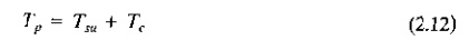
For job shop production when quantity Q=1, the production time per work unit is the sum of setup and operation cycle times:

For job shop production when the quantity is greater than one, then this reverts to the batch production case discussed above.

For quantity type mass production, we can say that the production rate equals the cycle rate of the machine (reciprocal of operation cycle time) after production is underway and the effects of setup time become insignificant. That is, as Q becomes very large, A T_su QB S 0 and

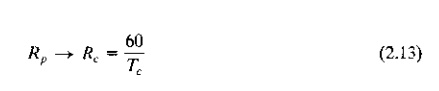
where R_c=operation cycle rate of the machine (pc hr), and T_c=operation cycle time (min pc).

For flow line mass production, the production rate approximates the cycle rate of the production line, again neglecting setup time. However, the operation of production lines is complicated by the interdependence of the workstations on the line. One complication is that it is usually impossible to divide the total work equally among all of the workstations on the line; therefore, one station ends up with the longest operation time, and this station sets the pace for the entire line. The term bottleneck station is sometimes used to refer to this station. Also included in the cycle time is the time to move parts from one station to the next at the end of each operation. In many production lines, all work units on the line are moved simultaneously, each to its respective next station. Taking these factors into account, the cycle time of a production line is the sum of the longest processing (or assembly) time plus the time to transfer work units between stations. This can be expressed:

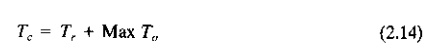
where T_c=cycle time of the production line (min cycle), T_r=time to transfer work units between stations each cycle (min pc), and Max T_o=operation time at the bottleneck station (the maximum of the operation times for all stations on the line, min cycle). Theoretically, the production rate can be determined by taking the reciprocal of T_c as follows:

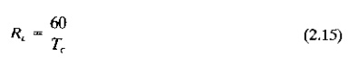
where R_c=theoretical or ideal production rate, but let us call it the cycle rate to be more precise (cycles hr), and T_c=ideal cycle time from Eq. (2.14) (min cycle).

Production lines are of two basic types: (1) manual and (2) automated. In the operation of automated production lines, another complicating factor is reliability. Poor reliability reduces the available production time on the line. This results from the interdependence of workstations in an automated line, in which the entire line is forced to stop when one station breaks down. The actual average production rate R_p is reduced to a value that is often substantially below the ideal R_c given by Eq. (2.15). We discuss reliability and some of its terminology in Section 2.4.3. The effect of reliability on automated production lines is examined in Chapters 18 and 19.

It is important to design the manufacturing method to be consistent with the pace at which the customer is demanding the part or product, sometimes referred to as the takt time (a German word for cadence or pace). The takt time is the reciprocal of demand rate, but adjusted for the available shift time in the factory. For example, if 100 product units were demanded from a customer each day, and the factory operated one shift day, with 400 min of time available per shift, then the takt time would be 400 min 100 units=4.0 min work unit.

  2 Production Capacity

We mentioned production capacity in our discussion of manufacturing capabilities (Section 2.3.3). Production capacity is defined as the maximum rate of output that a production facility (or production line, work center, or group of work centers) is able to produce under a given set of assumed operating conditions. The production facility usually refers to a plant or factory, and so the term plant capacity is often used for this measure. As mentioned before, the assumed operating conditions refer to the number of shifts per day (one, two, or three), number of days in the week (or month) that the plant operates, employment levels, and so forth.

The number of hours of plant operation per week is a critical issue in defining plant capacity. For continuous chemical production in which the reactions occur at elevated temperatures, the plant is usually operated 24 hr day, 7 day wk. For an automobile assembly plant, capacity is typically defined as one or two shifts. In the manufacture of discrete parts and products, a growing trend is to define plant capacity for the full 7day week, 24 hr day. This is the maximum time available (168 hr wk), and if the plant operates fewer hours than the maximum, then its maximum possible capacity is not being fully utilized.

Quantitative measures of plant capacity can be developed based on the production rate models derived earlier. Let PC=the production capacity of a given facility under consideration. Let the measure of capacity=the number of units produced per week. Let n=the number of machines or work centers in the facility. A work center is a manufacturing system in the plant typically consisting of one worker and one machine. It might also be one automated machine with no worker, or multiple workers working together on a production line. It is capable of producing at a rate R_p unit hr, as defined in Section 2.4.1. Each work center operates for H hr shift. Provision for setup time is included in R_p , according to Eq. (2.11). Let S denote the number of shifts per week. These parameters can be combined to calculate the production capacity of the facility:

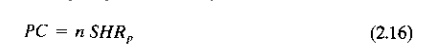
where PC=production capacity of the facility (output units wk), n=number of work centers producing in the facility, S=number of shifts per period (shift wk), H=hr shift (hr), and R_p=hourly production rate of each work center (output units hr). Although we have used a week as the time period of interest, Eq. (2.16) can easily be revised to adopt other periods (months, years, etc.). As in previous equations, our assumption is that the units processed through the group of work centers are homogeneous, and therefore the value of R_p is the same for all units produced.

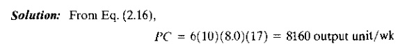
EXAMPLE 2.3               Production Capacity

The turret lathe section has six machines, all devoted to the production of the same part. The section operates 10 shift wk. The number of hours per shift averages 8.0. Average production rate of each machine is 17 unit hr. Determine the weekly production capacity of the turret lathe section.

If we include the possibility that each work unit is routed through n_o operations, with each operation requiring a new setup on either the same or different machine, then the plant capacity equation must be amended as follows:

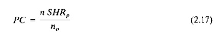
where n_o=number of distinct operations through which work units are routed, and the other terms have the same meaning as before.

Eq. (2.17) indicates the operating parameters that affect plant capacity. Changes that can be made to increase or decrease plant capacity over the short term are:

1. Change the number of shifts per week (S). For example, Saturday shifts might be authorized to temporarily increase capacity.

2. Change the number of hours worked per shift (H). For example, overtime on each regular shift might be authorized to increase capacity.

Over the intermediate or longer term, the following changes can be made to increase plant capacity:

3. Increase the number of work centers, n, in the shop. This might be done by using equipment that was formerly not in use and hiring new workers. Over the long term, new machines might be acquired. Decreasing capacity is easier, except for the social and economic impact: Workers must be laid off and machines decommissioned.

4. Increase the production rate, R_p by making improvements in methods or process technology.

5. Reduce the number of operations n_o required per work unit by using combined operations, simultaneous operations, or integration of operations (Section 1.5.2: strategies 2, 3, and 4).

This capacity model assumes that all n machines are producing 100% of the time, and there are no bottleneck operations due to variations in process routings to inhibit smooth flow of work through the plant. In real batch production machine shops where each product has a different operation sequence, it is unlikely that the work distribution among the productive resources (machines) can be perfectly balanced. Consequently, there are some operations that are fully utilized while other operations occasionally stand idle waiting for work. Let us examine the effect of utilization.

3 Utilization and Availability

Utilization refers to the amount of output of a production facility relative to its capacity. Expressing this as an equation,

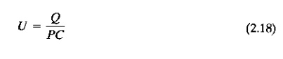
where U=utilization of the facility, Q=actual quantity produced by the facility during a given time period (i.e., pc wk), and PC=production capacity for the same period (pc wk).

Utilization can be assessed for an entire plant, a single machine in the plant, or any other productive resource (i.e., labor). For convenience, it is often defined as the proportion of time that the facility is operating relative to the time available under the definition of capacity. Utilization is usually expressed as a percentage.

EXAMPLE 2.4               Utilization

A production machine operates 80 hr wk (two shifts, 5 days) at full capacity. Its production rate is 20 unit hr. During a certain week, the machine produced 1000 parts and was idle the remaining time. (a) Determine the production capacity of the machine. (b) What was the utilization of the machine during the week under consideration?

Solution:                 (a) The capacity of the machine can be determined using the assumed 80hr week as follows:

PC=80(20)=1600 unit wk

(b) tilization can be determined as the ratio of the number of parts made by the machine relative to its capacity.

U=1000 1600=0.625                   (62.5%)

The alternative way of assessing utilization is by the time during the week that the machine was actually used. To produce 1000 units, the machine was operated

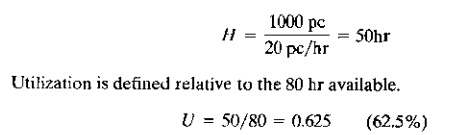
Availability is a common measure of reliability for equipment. It is especially appropriate for automated production equipment. Availability is defined using two other reliability terms, mean time between failure (MTBF) and mean time to repair (MTTR). The MTBF indicates the average length of time the piece of equipment runs between breakdowns. The MTTR indicates the average time required to service the equipment and put it back into operation when a breakdown occurs. Availability is defined as follows:

where A=availability, MTBF=mean time between failures (hr), and MTTR=mean time to repair (hr). Availability is typically expressed as a percentage. When a piece of equipment is brand new (and being debugged), and later when it begins to age, its availability tends to be lower.

EXAMPLE 2.5               Effect of Utilization and Availability on Plant Capacity

Consider previous Example 2.3. Suppose the same data from that example were applicable, but that the availability of the machines A=90%, and the utilization of the machines U=80%. Given this additional data, compute the expected plant output.

Solution:     Previous Eq. (2.16) can be altered to include availability and utilization as follows

where A=availability and U= utilization. Combining the previous and new data, we have

Q=0.90(0.80)(6)(10)(8.0)(17)=5875 output unit wk

4     Manufacturing Lead Time

In the competitive environment of modern business, the ability of a manufacturing firm to deliver a product to the customer in the shortest possible time often wins the order. This time is referred to as the manufacturing lead time. Specifically, we define manufacturing lead time (MLT) as the total time required to process a given part or product through the plant. Let us examine the components of MLT.

Production usually consists of a series of individual processing and assembly operations. Between the operations are material handling, storage, inspections, and other nonproductive activities. Let us therefore divide the activities of production into two main categories, operations and non-operation elements. An operation is performed on a work unit when it is in the production machine. The non-operation elements include handling, temporary storage, inspections, and other sources of delay when the work unit is not in the machine. Let T_c=the operation cycle time at a given machine or workstation, and T_no=the non-operation time associated with the same machine. Further, let us suppose that the number of separate operations (machines) through which the work unit must be routed to be completely processed=n_o . If we assume batch production, then there are Q work units in the batch. A setup is generally required to prepare each production machine for the particular product, which requires a time=T_su . Given these terms, we can define manufacturing lead time as:

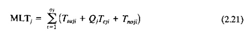
where MLT_j=manufacturing lead time for part or product j (min), T_suji=setup time for operation i (min), Q_j= quantity of part or product j in the batch being processed (pc),

T_cji=operation cycle time for operation i (min pc), T_noji= non operation time associated with operation i (min), and i indicates the operation sequence in the processing;

i=1, 2, p n_oj . The MLT equation does not include the time the raw workpart spends in storage before its turn in the production schedule begins.

To simplify and generalize our model, let us assume that all setup times, operation cycle times, and nonoperation times are equal for the n_oj machines. Further, let us suppose that the batch quantities of all parts or products processed through the plant are equal and that they are all processed through the same number of machines, so that n_oj=n_o. With these simplifications, Eq. (2.21) becomes:

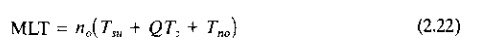
where MLT=average manufacturing lead time for a part or product (min).

In an actual batch production factory, which this equation is intended to represent, the terms n_o, Q, T_su, T_c, and T_no would vary by product and by operation. These variations can be accounted for by using properly weighted average values of the various terms. The averaging procedure is explained in the Appendix at the end of this chapter.

EXAMPLE 2.6               Manufacturing Lead Time

A certain part is produced in a batch size of 100 units. The batch must be routed through five operations to complete the processing of the parts. Average setup time is 3 hr operation, and average operation time is 6 min (0.1 hr). Average non operation time due to handling, delays, inspections, etc., is 7 hours for each operation. Determine how many days it will take to complete the batch, assuming the plant runs one 8hr shift day.

Solution:                 The manufacturing lead time is computed from Eq. (2.22)

MLT=5(3+100*0.1+7)=100 hours

At 8 hr day, this amounts to 100 8=12.5 days.

Eq. (2.22) can be adapted for job shop production and mass production by making adjustments in the parameter values. For a job shop in which the batch size is one (Q=1), Eq. (2.22) becomes

For mass production, the Q term in Eq. (2.22) is very large and dominates the other terms. In the case of quantity type mass production in which a large number of units are made on a single machine A n_o=1B , the MLT simply becomes the operation cycle time for the machine after the setup has been completed and production begins.

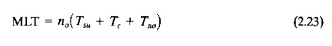
For flow line mass production, the entire production line is set up in advance. Also, the nonoperation time between processing steps is simply the transfer time T_r to move the part or product from one workstation to the next. If the workstations are integrated so that all stations are processing their own respective work units, then the time to accomplish all of the operations is the time it takes each work unit to progress through all of the stations on the line. The station with the longest operation time sets the pace for all stations.

where MLT=time between start and completion of a given work unit on the line (min), n_o=number of operations on the line; T_r=transfer time (min), Max T_o=operation time at the bottleneck station (min) and T_c=cycle time of the production line (min pc).

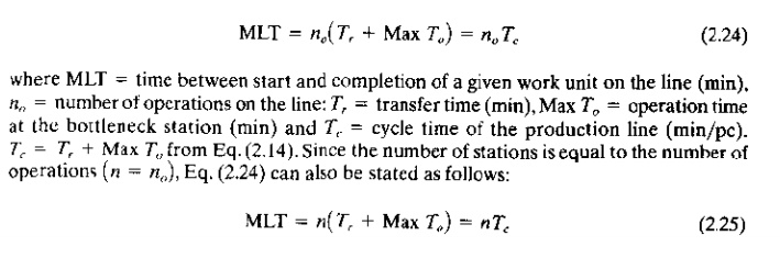
where the symbols have the same meaning as above, and we have substituted n (number of workstations or machines) for number of operations n_o .

5     Work-in-Process

Work-in-process (WIP) is the quantity of parts or products currently located in the factory that are either being processed or are between processing operations. WIP is inventory that is in the state of being transformed from raw material to finished product. An approximate measure of work-in-process can be obtained from the following, using terms previously defined:

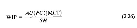
where WIP=workinprocess in the facility (pc), A=availability, U=utilization, PC=production capacity of the facility (pc wk), MLT=manufacturing lead time, (wk), S=number of shifts per week (shift wk), and H=hours per shift (hr shift). Eq. (2.26) states that the level of WIP equals the rate at which parts flow through the factory multiplied by the length of time the parts spend in the factory. The units for (PC) SH (e.g., pc wk) must be consistent with the units for MLT (e.g., weeks).

Work-in-process represents an investment by the firm, but one that cannot be turned into revenue until all processing has been completed. Many manufacturing companies sustain major costs because work remains in-process in the factory too long.