Problem Reduction

Problem Reduction

Here is my version of a well-known joke about mathematicians. Professor X, a noted mathematician, noticed that when his wife wanted to boil water for their tea, she took their kettle from their cupboard, filled it with water, and put it on the stove. Once, when his wife was away (if you have to know, she was signing her best-seller in a local bookstore), the professor had to boil water by himself. He saw that the kettle was sitting on the kitchen counter. What did Professor X do? He put the kettle in the cupboard first and then proceeded to follow his wife’s routine.

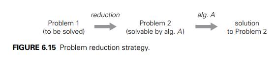
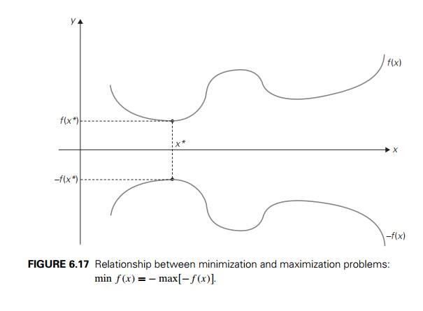
The way Professor X approached his task is an example of an important problem-solving strategy called problem reduction. If you need to solve a problem, reduce it to another problem that you know how to solve (Figure 6.15).

The joke about the professor notwithstanding, the idea of problem reduction plays a central role in theoretical computer science, where it is used to classify problems according to their complexity. We will touch on this classification in Chapter 11. But the strategy can be used for actual problem solving, too. The practical difficulty in applying it lies, of course, in finding a problem to which the problem at hand should be reduced. Moreover, if we want our efforts to be of practical value, we need our reduction-based algorithm to be more efficient than solving the original problem directly.

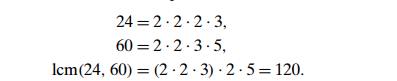
Note that we have already encountered this technique earlier in the book. In Section 6.5, for example, we mentioned the so-called synthetic division done by applying Horner’s rule for polynomial evaluation. In Section 5.5, we used the following fact from analytical geometry: if p₁(x₁, y₁), p₂(x₂, y₂), and p₃(x₃, y₃) are three arbitrary points in the plane, then the determinant

is positive if and only if the point p₃ is to the left of the directed line p₁p₂ through points p₁ and p₂. In other words, we reduced a geometric question about the relative locations of three points to a question about the sign of a determinant. In fact, the entire idea of analytical geometry is based on reducing geometric problems to algebraic ones. And the vast majority of geometric algorithms take advantage of this historic insight by Rene´ Descartes (1596–1650). In this section, we give a few more examples of algorithms based on the strategy of problem reduction.

Computing the Least Common Multiple

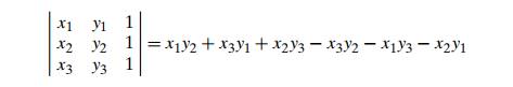
Recall that the least common multiple of two positive integers m and n, denoted lcm(m, n), is defined as the smallest integer that is divisible by both m and n. For example, lcm(24, 60) = 120, and lcm(11, 5) = 55. The least common multiple is one of the most important notions in elementary arithmetic and algebra. Perhaps you remember the following middle-school method for computing it: Given the prime factorizations of m and n, compute the product of all the common prime factors of m and n, all the prime factors of m that are not in n, and all the prime factors of n that are not in m. For example,

lcm(24, 60) = (2 ^. 2 ^. 3) ^. 2 ^. 5 = 120.

As a computational procedure, this algorithm has the same drawbacks as the middle-school algorithm for computing the greatest common divisor discussed in Section 1.1: it is inefficient and requires a list of consecutive primes.

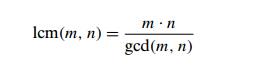
A much more efficient algorithm for computing the least common multiple can be devised by using problem reduction. After all, there is a very efficient algorithm (Euclid’s algorithm) for finding the greatest common divisor, which is a product of all the common prime factors of m and n. Can we find a formula relating lcm(m, n) and gcd(m, n)? It is not difficult to see that the product of lcm(m, n) and gcd(m, n) includes every factor of m and n exactly once and hence is simply equal to the product of m and n. This observation leads to the formula

where gcd(m, n) can be computed very efficiently by Euclid’s algorithm.

Counting Paths in a Graph

As our next example, we consider the problem of counting paths between two vertices in a graph. It is not difficult to prove by mathematical induction that the number of different paths of length k > 0 from the ith vertex to the j th vertex of a graph (undirected or directed) equals the (i, j )th element of A^k where A is the adjacency matrix of the graph. Therefore, the problem of counting a graph’s paths can be solved with an algorithm for computing an appropriate power of its adjacency matrix. Note that the exponentiation algorithms we discussed before for computing powers of numbers are applicable to matrices as well.

As a specific example, consider the graph of Figure 6.16. Its adjacency matrix A and its square A² indicate the numbers of paths of length 1 and 2, respectively, between the corresponding vertices of the graph. In particular, there are three

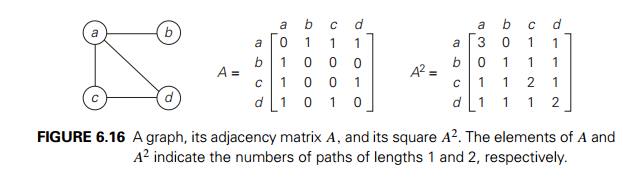
paths of length 2 that start and end at vertex a (a − b − a, a − c − a, and a − d − a); but there is only one path of length 2 from a to c (a − d − c).

Reduction of Optimization Problems

Our next example deals with solving optimization problems. If a problem asks to find a maximum of some function, it is said to be a maximization problem; if it asks to find a function’s minimum, it is called a minimization problem. Suppose now that you need to find a minimum of some function f (x) and you have an algorithm for function maximization. How can you take advantage of the latter? The answer lies in the simple formula

min f (x) = − max[−f (x)].

In other words, to minimize a function, we can maximize its negative instead and, to get a correct minimal value of the function itself, change the sign of the answer. This property is illustrated for a function of one real variable in Figure 6.17.

Of course, the formula

max f (x) = − min[−f (x)]

is valid as well; it shows how a maximization problem can be reduced to an equivalent minimization problem.

This relationship between minimization and maximization problems is very general: it holds for functions defined on any domain D. In particular, we can

apply it to functions of several variables subject to additional constraints. A very important class of such problems is introduced below in this section.

Now that we are on the topic of function optimization, it is worth pointing out that the standard calculus procedure for finding extremum points of a function is, in fact, also based on problem reduction. Indeed, it suggests finding the function’s derivative f (x) and then solving the equation f (x) = 0 to find the function’s critical points. In other words, the optimization problem is reduced to the problem of solving an equation as the principal part of finding extremum points. Note that we are not calling the calculus procedure an algorithm, since it is not clearly defined. In fact, there is no general method for solving equations. A little secret of calculus textbooks is that problems are carefully selected so that critical points can always be found without difficulty. This makes the lives of both students and instructors easier but, in the process, may unintentionally create a wrong impression in students’ minds.

Linear Programming

Many problems of optimal decision making can be reduced to an instance of the linear programming problem—a problem of optimizing a linear function of several variables subject to constraints in the form of linear equations and linear inequalities.

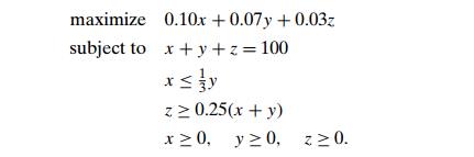
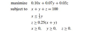
EXAMPLE 1 Consider a university endowment that needs to invest $100 million. This sum has to be split between three types of investments: stocks, bonds, and cash. The endowment managers expect an annual return of 10%, 7%, and 3% for their stock, bond, and cash investments, respectively. Since stocks are more risky than bonds, the endowment rules require the amount invested in stocks to be no more than one-third of the moneys invested in bonds. In addition, at least 25% of the total amount invested in stocks and bonds must be invested in cash. How should the managers invest the money to maximize the return?

Let us create a mathematical model of this problem. Let x, y, and z be the amounts (in millions of dollars) invested in stocks, bonds, and cash, respectively. By using these variables, we can pose the following optimization problem:

Although this example is both small and simple, it does show how a problem of optimal decision making can be reduced to an instance of the general linear programming problem

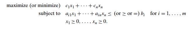
(The last group of constraints—called the nonnegativity constraints—are, strictly speaking, unnecessary because they are special cases of more general constraints a_i1x₁ + ^{. . .} + a_inx_n ≥ b_i, but it is convenient to treat them separately.)

Linear programming has proved to be flexible enough to model a wide variety of important applications, such as airline crew scheduling, transportation and communication network planning, oil exploration and refining, and industrial production optimization. In fact, linear programming is considered by many as one of the most important achievements in the history of applied mathematics.

The classic algorithm for this problem is called the simplex method (Sec-tion 10.1). It was discovered by the U.S. mathematician George Dantzig in the 1940s [Dan63]. Although the worst-case efficiency of this algorithm is known to be exponential, it performs very well on typical inputs. Moreover, a more recent al-gorithm by Narendra Karmarkar [Kar84] not only has a proven polynomial worst-case efficiency but has also performed competitively with the simplex method in empirical tests.

It is important to stress, however, that the simplex method and Karmarkar’s algorithm can successfully handle only linear programming problems that do not limit its variables to integer values. When variables of a linear programming problem are required to be integers, the linear programming problem is said to be an integer linear programming problem. Except for some special cases (e.g., the assignment problem and the problems discussed in Sections 10.2–10.4), integer linear programming problems are much more difficult. There is no known polynomial-time algorithm for solving an arbitrary instance of the general integer linear programming problem and, as we see in Chapter 11, such an algorithm quite possibly does not exist. Other approaches such as the branch-and-bound technique discussed in Section 12.2 are typically used for solving integer linear programming problems.

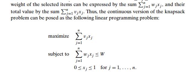
EXAMPLE 2 Let us see how the knapsack problem can be reduced to a linear programming problem. Recall from Section 3.4 that the knapsack problem can be posed as follows. Given a knapsack of capacity W and n items of weights w₁, . . . , w_n and values v₁, . . . , v_n, find the most valuable subset of the items that fits into the knapsack. We consider first the continuous (or fractional) version of the problem, in which any fraction of any item given can be taken into the knapsack. Let x_j , j = 1, . . . , n, be a variable representing a fraction of item j taken into the knapsack. Obviously, x_j must satisfy the inequality 0 ≤ x_j ≤ 1. Then the total

EXAMPLE 2 Let us see how the knapsack problem can be reduced to a linear programming problem. Recall from Section 3.4 that the knapsack problem can be posed as follows. Given a knapsack of capacity W and n items of weights w1, . . . , wn and values v1, . . . , vn, find the most valuable subset of the items that fits into the knapsack. We consider first the continuous (or fractional) version of the problem, in which any fraction of any item given can be taken into the knapsack. Let xj , j = 1, . . . , n, be a variable representing a fraction of item j taken into the knapsack. Obviously, xj must satisfy the inequality 0 ≤ xj ≤ 1. Then the total

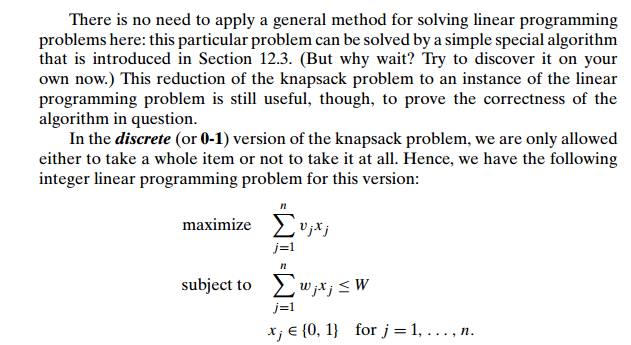
This seemingly minor modification makes a drastic difference for the com-plexity of this and similar problems constrained to take only discrete values in their potential ranges. Despite the fact that the 0-1 version might seem to be eas-ier because it can ignore any subset of the continuous version that has a fractional value of an item, the 0-1 version is, in fact, much more complicated than its con-tinuous counterpart. The reader interested in specific algorithms for solving this problem will find a wealth of literature on the subject, including the monographs [Mar90] and [Kel04].

Reduction to Graph Problems

As we pointed out in Section 1.3, many problems can be solved by a reduction to one of the standard graph problems. This is true, in particular, for a variety of puzzles and games. In these applications, vertices of a graph typically represent possible states of the problem in question, and edges indicate permitted transi-tions among such states. One of the graph’s vertices represents an initial state and another represents a goal state of the problem. (There might be several vertices of the latter kind.) Such a graph is called a state-space graph. Thus, the transfor-mation just described reduces the problem to the question about a path from the initial-state vertex to a goal-state vertex.

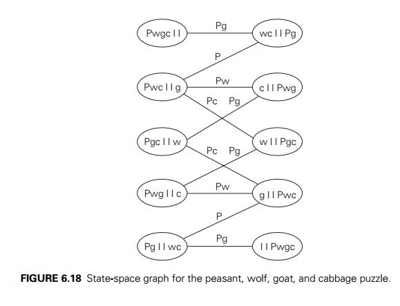
EXAMPLE Let us revisit the classic river-crossing puzzle that was included in the exercises for Section 1.2. A peasant finds himself on a river bank with a wolf, a goat, and a head of cabbage. He needs to transport all three to the other side of the river in his boat. However, the boat has room only for the peasant himself and one other item (either the wolf, the goat, or the cabbage). In his absence, the wolf would eat the goat, and the goat would eat the cabbage. Find a way for the peasant to solve his problem or prove that it has no solution.

The state-space graph for this problem is given in Figure 6.18. Its vertices are labeled to indicate the states they represent: P, w, g, c stand for the peasant, the wolf, the goat, and the cabbage, respectively; the two bars | | denote the river; for convenience, we also label the edges by indicating the boat’s occupants for each crossing. In terms of this graph, we are interested in finding a path from the initial-state vertex labeled Pwgc| | to the final-state vertex labeled | |Pwgc.

It is easy to see that there exist two distinct simple paths from the initial-state vertex to the final state vertex (what are they?). If we find them by applying breadth-first search, we get a formal proof that these paths have the smallest number of edges possible. Hence, this puzzle has two solutions requiring seven river crossings, which is the minimum number of crossings needed.

Our success in solving this simple puzzle should not lead you to believe that generating and investigating state-space graphs is always a straightforward task. To get a better appreciation of them, consult books on artificial intelligence (AI), the branch of computer science in which state-space graphs are a principal subject.

In this book, we deal with an important special case of state-space graphs in Sections 12.1 and 12.2.

Exercises 6.6

1. a.  Prove the equality

that underlies the algorithm for computing lcm(m, n).

            Euclid’s algorithm is known to be in O(log n). If it is the algorithm that is used for computing gcd(m, n), what is the efficiency of the algorithm for computing lcm(m, n)?

            You are given a list of numbers for which you need to construct a min-heap. (A min-heap is a complete binary tree in which every key is less than or equal to the keys in its children.) How would you use an algorithm for constructing a max-heap (a heap as defined in Section 6.4) to construct a min-heap?

            Prove that the number of different paths of length k > 0 from the ith vertex to the j th vertex in a graph (undirected or directed) equals the (i, j )th element of A^k where A is the adjacency matrix of the graph.

            a. Design an algorithm with a time efficiency better than cubic for checking whether a graph with n vertices contains a cycle of length 3 [Man89].

            Consider the following algorithm for the same problem. Starting at an arbi-trary vertex, traverse the graph by depth-first search and check whether its depth-first search forest has a vertex with a back edge leading to its grand-parent. If it does, the graph contains a triangle; if it does not, the graph does not contain a triangle as its subgraph. Is this algorithm correct?

            Given n > 3 points P₁ = (x₁, y₁), . . . , P_n = (x_n, y_n) in the coordinate plane, design an algorithm to check whether all the points lie within a triangle with its vertices at three of the points given. (You can either design an algorithm from scratch or reduce the problem to another one with a known algorithm.)

            Consider the problem of finding, for a given positive integer n, the pair of integers whose sum is n and whose product is as large as possible. Design an efficient algorithm for this problem and indicate its efficiency class.

7. The assignment problem introduced in Section 3.4 can be stated as follows: There are n people who need to be assigned to execute n jobs, one person per job. (That is, each person is assigned to exactly one job and each job is assigned to exactly one person.) The cost that would accrue if the ith person is assigned to the j th job is a known quantity C[i, j ] for each pair i, j = 1, . . . , n. The problem is to assign the people to the jobs to minimize the total cost of the assignment. Express the assignment problem as a 0-1 linear programming problem.

8. Solve the instance of the linear programming problem given in Section 6.6:

          9.   The graph-coloring problem is usually stated as the vertex-coloring prob-lem: Assign the smallest number of colors to vertices of a given graph so that no two adjacent vertices are the same color. Consider the edge-coloring problem: Assign the smallest number of colors possible to edges of a given graph so that no two edges with the same endpoint are the same color. Ex-plain how the edge-coloring problem can be reduced to a vertex-coloring problem.

       11.      Jealous husbands There are n ≥ 2 married couples who need to cross a river. They have a boat that can hold no more than two people at a time. To complicate matters, all the husbands are jealous and will not agree on any crossing procedure that would put a wife on the same bank of the river with another woman’s husband without the wife’s husband being there too, even if there are other people on the same bank. Can they cross the river under such constraints?

            Solve the problem for n = 2.

            Solve the problem for n = 3, which is the classical version of this problem.

            Does the problem have a solution for n ≥ 4? If it does, indicate how many river crossings it will take; if it does not, explain why.

12. Double-n dominoes Dominoes are small rectangular tiles with dots called spots or pips embossed at both halves of the tiles. A standard “double-six” domino set has 28 tiles: one for each unordered pair of integers from (0, 0) to (6, 6). In general, a “double-n” domino set would consist of domino tiles for each unordered pair of integers from (0, 0) to (n, n). Determine all values of n for which one constructs a ring made up of all the tiles in a double-n domino set.