Chapter: Introduction to the Design and Analysis of Algorithms : Transform and Conquer
Balanced Search Trees: AVL Trees and 2-3 Trees
Balanced Search
Trees
In Sections 1.4, 4.5, and 5.3, we discussed the
binary search treeŌĆöone of the prin-cipal data structures for implementing
dictionaries. It is a binary tree whose nodes contain elements of a set of
orderable items, one element per node, so that all ele-ments in the left
subtree are smaller than the element in the subtreeŌĆÖs root, and all the
elements in the right subtree are greater than it. Note that this
transformation from a set to a binary search tree is an example of the
representation-change tech-nique. What do we gain by such transformation
compared to the straightforward implementation of a dictionary by, say, an
array? We gain in the time efficiency of searching, insertion, and deletion,
which are all in (log n), but only in the av-erage case. In the worst
case, these operations are in (n) because the tree can degenerate into a severely unbalanced one
with its height equal to n ŌłÆ 1.
Computer scientists have expended a lot of
effort in trying to find a structure that preserves the good properties of the
classical binary search treeŌĆöprincipally, the logarithmic efficiency of the
dictionary operations and having the setŌĆÖs ele-ments sortedŌĆöbut avoids its
worst-case degeneracy. They have come up with two approaches.
The first approach is of the
instance-simplification variety: an unbalanced binary search tree is
transformed into a balanced one. Because of this, such trees are called self-balancing.
Specific implementations of this idea differ by their definition of balance. An
AVL
tree requires the difference between the heights of the left and right
subtrees of every node never exceed 1. A red-black tree tolerates the height
of one subtree being twice as large as the other subtree of the same node. If
an insertion or deletion of a new node creates a tree with a violated balance
requirement, the tree is restructured by one of a family of special
transformations called rotations that restore the balance
required. In this section, we will discuss only AVL trees. Information about
other types of binary search trees that utilize the idea of rebalancing via
rotations, including red-black trees and splay trees, can be found in the
references [Cor09], [Sed02], and [Tar83].
The second approach is of the
representation-change variety: allow more than one element in a node of a
search tree. Specific cases of such trees are 2-3 trees,
2-3-4 trees, and more general and important B-trees. They differ in the number
of elements admissible in a single node of a search tree, but all are perfectly
balanced. We discuss the simplest case of such trees, the 2-3 tree, in this
section, leaving the discussion of B-trees
for Chapter 7.
AVL Trees
AVL trees were invented in 1962 by two Russian
scientists, G. M. Adelson-Velsky and E. M. Landis [Ade62], after whom this data
structure is named.
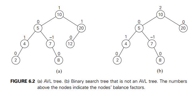
DEFINITION An AVL tree is a binary search tree in which the balance factor of every node, which is defined as the difference between the heights
of the nodeŌĆÖs left and right subtrees, is either 0 or +1 or ŌłÆ1. (The height of the empty tree is defined as ŌłÆ1. Of course, the balance factor can also be computed as the
difference between the numbers of levels rather than the height difference of
the nodeŌĆÖs left and right subtrees.)
For example, the binary search tree in Figure
6.2a is an AVL tree but the one in Figure 6.2b is not.
If an insertion of a new node makes an AVL tree
unbalanced, we transform the tree by a rotation. A rotation in an AVL tree
is a local transformation of its subtree rooted at a node whose balance has
become either +2 or ŌłÆ2. If there are several such nodes, we rotate
the tree rooted at the unbalanced node that is the closest to the newly
inserted leaf. There are only four types of rotations; in fact, two of them are
mirror images of the other two. In their simplest form, the four rotations are
shown in Figure 6.3.
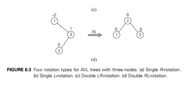
The first rotation type is called the single
right rotation, or R-rotation. (Imag-ine rotating the
edge connecting the root and its left child in the binary tree in Figure 6.3a
to the right.) Figure 6.4 presents the single R-rotation in its most gen-eral form. Note that this rotation is
performed after a new key is inserted into the left subtree of the left child
of a tree whose root had the balance of +1 before the insertion.
The symmetric single left rotation, or L-rotation,
is the mirror image of the single R-rotation. It is performed after a new key is
inserted into the right subtree of the right child of a tree whose root had the
balance of ŌłÆ1 before the insertion. (You are asked to draw a diagram of the
general case of the single L-rotation in the exercises.)
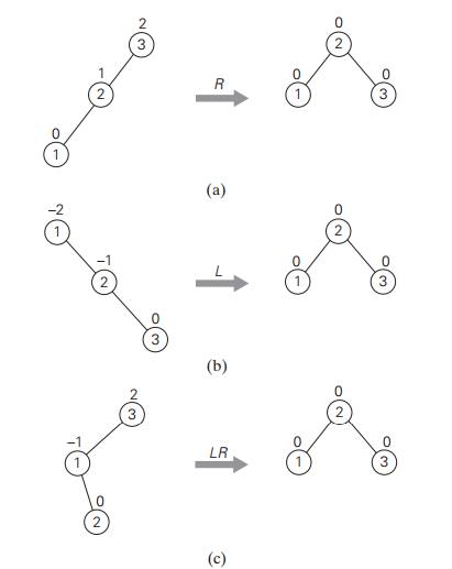
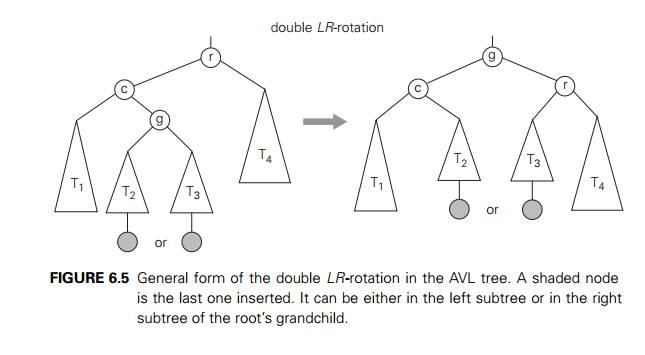
The second rotation type is called the double
left-right rotation (LR-rotation). It is, in fact, a
combination of two rotations: we perform the L-rotation of the left subtree of root r followed by the R-rotation
of the new tree rooted at r (Figure 6.5). It is performed after a new key
is inserted into the right subtree of the left child of a tree whose root had the
balance of +1 before the insertion.
The double right-left rotation (RL-rotation)
is the mirror image of the double
LR-rotation and is left for the exercises.
Note that the rotations are not trivial
transformations, though fortunately they can be done in constant time. Not only
should they guarantee that a resulting tree is balanced, but they should also
preserve the basic requirements of a binary search tree. For example, in the
initial tree of Figure 6.4, all the keys of subtree T1 are smaller than c, which is smaller than all the keys of subtree T2, which are smaller than r, which is smaller than all the keys of subtree T3. And the same relationships among the key
values hold, as they must, for the balanced tree after the rotation.
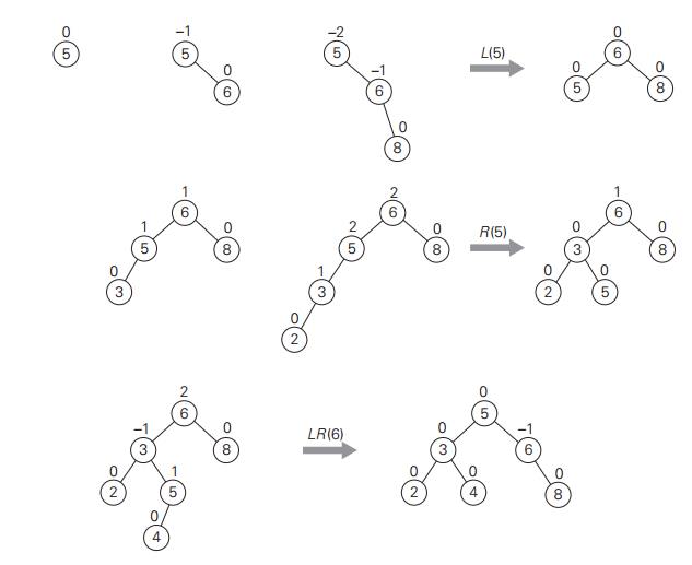
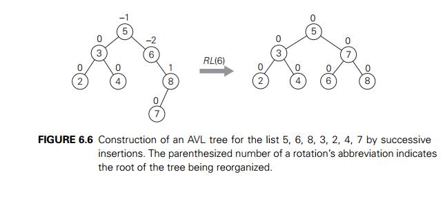
An example of constructing an AVL tree for a
given list of numbers is shown in Figure 6.6. As you trace the algorithmŌĆÖs
operations, keep in mind that if there are several nodes with the ┬▒2 balance, the rotation is done for the tree rooted at the
unbalanced node that is the closest to the newly inserted leaf.
How efficient are AVL trees? As with any search
tree, the critical charac-teristic is the treeŌĆÖs height. It turns out that it
is bounded both above and below
by logarithmic functions. Specifically, the
height h of any AVL tree with n nodes satisfies the inequalities
log2 n Ōēż h < 1.4405 log2(n + 2) ŌłÆ 1.3277.
(These weird-looking constants are round-offs
of some irrational numbers related to Fibonacci numbers and the golden
ratioŌĆösee Section 2.5.)
The inequalities immediately imply that the
operations of searching and in-sertion are (log n) in the worst case. Getting an exact formula
for the average height of an AVL tree constructed for random lists of keys has
proved to be dif-ficult, but it is known from extensive experiments that it is
about 1.01log2 n + 0.1 except when n is small [KnuIII, p. 468]. Thus, searching in
an AVL tree requires, on average, almost the same number of comparisons as
searching in a sorted array by binary search.
The operation of key deletion in an AVL tree is
considerably more difficult than insertion, but fortunately it turns out to be
in the same efficiency class as insertion, i.e., logarithmic.
These impressive efficiency characteristics
come at a price, however. The drawbacks of AVL trees are frequent rotations and
the need to maintain bal-ances for its nodes. These drawbacks have prevented
AVL trees from becoming the standard structure for implementing dictionaries.
At the same time, their un-derlying ideaŌĆöthat of rebalancing a binary search
tree via rotationsŌĆöhas proved to be very fruitful and has led to discoveries of
other interesting variations of the classical binary search tree.
2-3 Trees
As mentioned at the beginning of this section,
the second idea of balancing a search tree is to allow more than one key in the
same node of such a tree. The simplest implementation of this idea is 2-3
trees, introduced by the U.S. computer scientist John Hopcroft in 1970. A 2-3
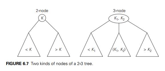
tree is a tree that can have nodes of two kinds: 2-nodes and 3-nodes. A
2-node
contains a single key K and has two children: the left child serves as
the root of a subtree whose keys are less than K, and the right child serves as the root of a
subtree whose keys are greater than K. (In other words, a 2-node is the same kind of
node we have in the classical binary search tree.) A 3-node contains two
ordered keys K1 and K2 (K1 < K2) and has three children. The leftmost child
serves as the root of a subtree with keys less than K1, the middle child serves as the root of a subtree with keys
between K1 and K2, and the rightmost child serves as the root of
a subtree with keys greater than K2 (Figure 6.7).
The last requirement of the 2-3 tree is that
all its leaves must be on the same level. In other words, a 2-3 tree is always
perfectly height-balanced: the length of a path from the root to a leaf is the
same for every leaf. It is this property that we ŌĆ£buyŌĆØ by allowing more than
one key in the same node of a search tree.
Searching for a given key K in a 2-3 tree is quite straightforward. We start at the root. If
the root is a 2-node, we act as if it were a binary search tree: we either stop
if K is equal to the rootŌĆÖs key or continue the search in the left or
right
subtree if K is, respectively, smaller or larger than the
rootŌĆÖs key. If the root is a 3-node, we know after no more than two key
comparisons whether the search can be stopped (if K is equal to one of the rootŌĆÖs keys) or in
which of the rootŌĆÖs three subtrees it needs to be continued.
Inserting a new key in a 2-3 tree is done as
follows. First of all, we always insert a new key K in a leaf, except for the empty tree. The
appropriate leaf is found by performing a search for K. If the leaf in question is a 2-node, we insert K there as either the first or the second key, depending on whether K is smaller or larger than the nodeŌĆÖs old key. If the leaf is
a 3-node, we split the leaf in two: the smallest of the three keys (two old
ones and the new key) is put in the first leaf, the largest key is put in the
second leaf, and the middle key is promoted to the old leafŌĆÖs parent. (If the
leaf happens to be the treeŌĆÖs root, a new root is created to accept the middle
key.) Note that promotion of a middle key to its parent can cause the parentŌĆÖs
overflow (if it was a 3-node) and hence can lead to several node splits along
the chain of the leafŌĆÖs ancestors.
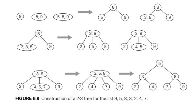
An example of a 2-3 tree construction is given
in Figure 6.8.
As for any search tree, the efficiency of the
dictionary operations depends on the treeŌĆÖs height. So let us first find an
upper bound for it. A 2-3 tree of height h with the smallest number of keys is a full
tree of 2-nodes (such as the final tree in Figure 6.8 for h = 2). Therefore, for any 2-3 tree of height h with n nodes, we get the inequality
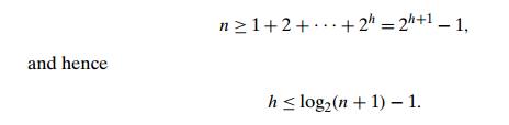
On the other hand, a 2-3 tree of height h with the largest number of keys is a full tree of 3-nodes, each
with two keys and three children. Therefore, for any 2-3 tree with n nodes,
n Ōēż 2 . 1 + 2 . 3 + . . . + 2 . 3h = 2(1 + 3 + .
. . + 3h) = 3h+1 ŌĆō 1
and hence
h Ōēź log3(n + 1) ŌłÆ 1.
These lower and upper bounds on height h,
log3(n + 1) ŌłÆ 1 Ōēż h Ōēż log2(n + 1) ŌłÆ 1,
imply that the time efficiencies of searching,
insertion, and deletion are all in (log n) in both the worst and average case. We consider
a very important gener-alization of 2-3 trees, called B-trees, in Section 7.4.
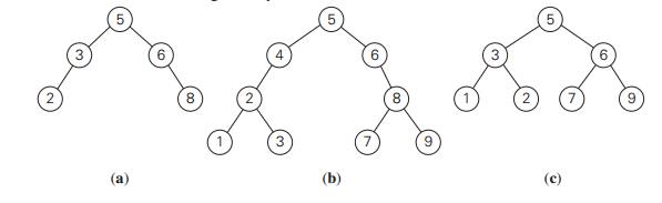
1. Which of the following binary trees are AVL
trees?
a. For n = 1, 2, 3, 4, and 5, draw all the binary trees with n nodes that satisfy the balance requirement of AVL trees.
Draw a
binary tree of height 4 that can be an AVL tree and has the smallest number of
nodes among all such trees.
Draw
diagrams of the single L-rotation and
of the double RL-rotation in their
general form.
For each
of the following lists, construct an AVL tree by inserting their ele-ments
successively, starting with the empty tree.
1, 2, 3,
4, 5, 6
6, 5, 4,
3, 2, 1
3, 6, 5,
1, 2, 4
a. For an AVL tree containing real numbers, design an algorithm for comput-ing
the range (i.e., the difference between the largest and smallest numbers in the
tree) and determine its worst-case efficiency.
True or
false: The smallest and the largest keys in an AVL tree can always be found on
either the last level or the next-to-last level?
Write a
program for constructing an AVL tree for a given list of n distinct integers.
a. Construct a 2-3 tree for the list C, O, M, P, U, T, I, N, G. Use
the alphabetical order of the
letters and insert them successively starting with the empty tree.
Assuming
that the probabilities of searching for each of the keys (i.e., the letters)
are the same, find the largest number and the average number of key comparisons
for successful searches in this tree.
Let TB and T2-3 be, respectively, a classical binary search tree and a 2-3 tree
constructed for the same list of keys inserted in the corresponding trees in
the same order. True or false: Searching for the same key in T2-3 always
takes fewer or the same number of key comparisons as searching in TB ?
For a
2-3 tree containing real numbers, design an algorithm for computing the range
(i.e., the difference between the largest and smallest numbers in the tree) and
determine its worst-case efficiency.
Write a
program for constructing a 2-3 tree for a given list of n integers.
Related Topics