Heaps and Heapsort

Heaps and Heapsort

The data structure called the “heap” is definitely not a disordered pile of items as the word’s definition in a standard dictionary might suggest. Rather, it is a clever, partially ordered data structure that is especially suitable for implementing priority queues. Recall that a priority queue is a multiset of items with an orderable characteristic called an item’s priority, with the following operations:

finding an item with the highest (i.e., largest) priority deleting an item with the highest priority

adding a new item to the multiset

It is primarily an efficient implementation of these operations that makes the heap both interesting and useful. Priority queues arise naturally in such ap-plications as scheduling job executions by computer operating systems and traf-fic management by communication networks. They also arise in several impor-tant algorithms, e.g., Prim’s algorithm (Section 9.1), Dijkstra’s algorithm (Sec-tion 9.3), Huffman encoding (Section 9.4), and branch-and-bound applications (Section 12.2). The heap is also the data structure that serves as a cornerstone of a theoretically important sorting algorithm called heapsort. We discuss this algo-rithm after we define the heap and investigate its basic properties.

Notion of the Heap

DEFINITION A heap can be defined as a binary tree with keys assigned to its nodes, one key per node, provided the following two conditions are met:

            The shape property—the binary tree is essentially complete (or simply com-plete), i.e., all its levels are full except possibly the last level, where only some rightmost leaves may be missing.

            The parental dominance or heap property—the key in each node is greater than or equal to the keys in its children. (This condition is considered auto-matically satisfied for all leaves.)⁵

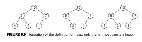
For example, consider the trees of Figure 6.9. The first tree is a heap. The second one is not a heap, because the tree’s shape property is violated. And the third one is not a heap, because the parental dominance fails for the node with key 5.

Note that key values in a heap are ordered top down; i.e., a sequence of values on any path from the root to a leaf is decreasing (nonincreasing, if equal keys are allowed). However, there is no left-to-right order in key values; i.e., there is no

relationship among key values for nodes either on the same level of the tree or, more generally, in the left and right subtrees of the same node.

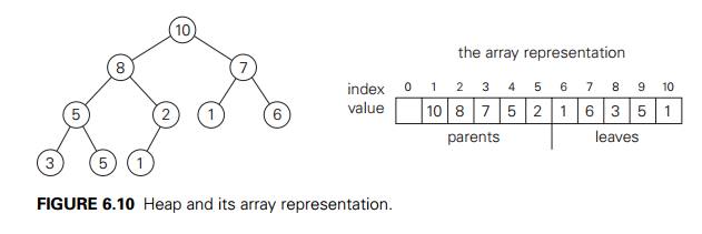
Here is a list of important properties of heaps, which are not difficult to prove (check these properties for the heap of Figure 6.10, as an example).

            There exists exactly one essentially complete binary tree with n nodes. Its height is equal to log₂ n .

            The root of a heap always contains its largest element.

            A node of a heap considered with all its descendants is also a heap.

            A heap can be implemented as an array by recording its elements in the top-down, left-to-right fashion. It is convenient to store the heap’s elements in positions 1 through n of such an array, leaving H [0] either unused or putting there a sentinel whose value is greater than every element in the heap. In such a representation,

            the parental node keys will be in the first n/2 positions of the array, while the leaf keys will occupy the last n/2 positions;

            the children of a key in the array’s parental position i (1 ≤ i ≤ n/2 ) will be in positions 2i and 2i + 1, and, correspondingly, the parent of a key in position i (2 ≤ i ≤ n) will be in position i/2 .

Thus, we could also define a heap as an array H [1..n] in which every element in position i in the first half of the array is greater than or equal to the elements in positions 2i and 2i + 1, i.e.,

H [i] ≥ max{H [2i], H [2i + 1]}      for i = 1, . . . ,  n/2 .

(Of course, if 2i + 1 > n, just H [i] ≥ H [2i] needs to be satisfied.) While the ideas behind the majority of algorithms dealing with heaps are easier to understand if we think of heaps as binary trees, their actual implementations are usually much simpler and more efficient with arrays.

How can we construct a heap for a given list of keys? There are two principal alternatives for doing this. The first is the bottom-up heap construction algorithm illustrated in Figure 6.11. It initializes the essentially complete binary tree with n nodes by placing keys in the order given and then “heapifies” the tree as follows. Starting with the last parental node, the algorithm checks whether the parental

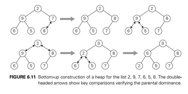
dominance holds for the key in this node. If it does not, the algorithm exchanges the node’s key K with the larger key of its children and checks whether the parental dominance holds for K in its new position. This process continues until the parental dominance for K is satisfied. (Eventually, it has to because it holds automatically for any key in a leaf.) After completing the “heapification” of the subtree rooted at the current parental node, the algorithm proceeds to do the same for the node’s immediate predecessor. The algorithm stops after this is done for the root of the tree.

ALGORITHM     HeapBottomUp(H [1..n])

//Constructs a heap from elements of a given array // by the bottom-up algorithm

//Input: An array H [1..n] of orderable items //Output: A heap H [1..n]

for i ← n/2 downto 1 do k ← i; v ← H [k] heap ← false

while not heap and 2 ∗ k ≤ n do

j ← 2 ∗ k

if j < n //there are two children if H [j ] < H [j + 1] j ← j + 1

if v ≥ H [j ]

heap ← true

else H [k] ← H [j ]; k ← j H [k] ← v

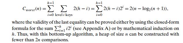
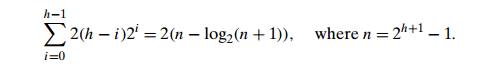
How efficient is this algorithm in the worst case? Assume, for simplicity, that n = 2^k − 1 so that a heap’s tree is full, i.e., the largest possible number of nodes occurs on each level. Let h be the height of the tree. According to the first property of heaps in the list at the beginning of the section, h = log₂ n or just log₂ (n + 1) − 1 = k − 1 for the specific values of n we are considering. Each key on level i of the tree will travel to the leaf level h in the worst case of the heap construction algorithm. Since moving to the next level down requires two comparisons—one to find the larger child and the other to determine whether the exchange is required—the total number of key comparisons involving a key on level i will be 2(h − i). Therefore, the total number of key comparisons in the worst case will be

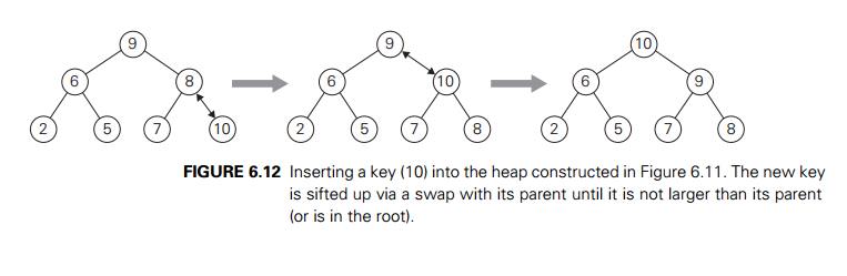
The alternative (and less efficient) algorithm constructs a heap by successive insertions of a new key into a previously constructed heap; some people call it the top-down heap construction algorithm. So how can we insert a new key K into a heap? First, attach a new node with key K in it after the last leaf of the existing heap. Then sift K up to its appropriate place in the new heap as follows. Compare K with its parent’s key: if the latter is greater than or equal to K, stop (the structure is a heap); otherwise, swap these two keys and compare K with its new parent. This swapping continues until K is not greater than its last parent or it reaches the root (illustrated in Figure 6.12).

Obviously, this insertion operation cannot require more key comparisons than the heap’s height. Since the height of a heap with n nodes is about log₂ n, the time efficiency of insertion is in O(log n).

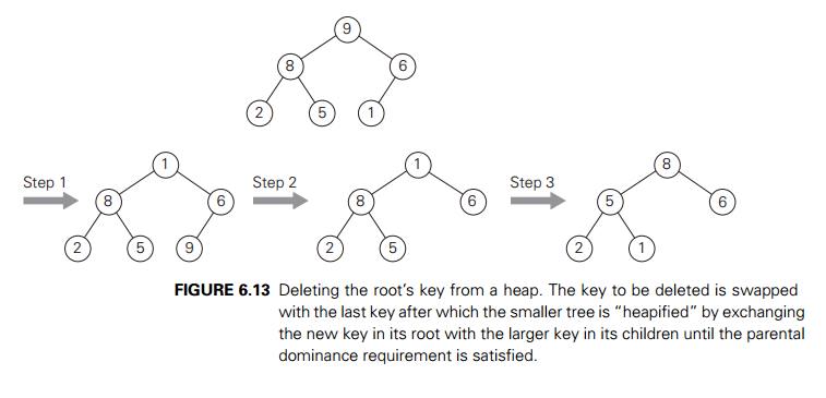
How can we delete an item from a heap? We consider here only the most important case of deleting the root’s key, leaving the question about deleting an arbitrary key in a heap for the exercises. (Authors of textbooks like to do such things to their readers, do they not?) Deleting the root’s key from a heap can be done with the following algorithm, illustrated in Figure 6.13.

Maximum Key Deletion from a heap

Step 1 Exchange the root’s key with the last key K of the heap. Step 2 Decrease the heap’s size by 1.

Step 3 “Heapify” the smaller tree by sifting K down the tree exactly in the same way we did it in the bottom-up heap construction algorithm. That is, verify the parental dominance for K: if it holds, we are done; if not, swap K with the larger of its children and repeat this operation until the parental dominance condition holds for K in its new position.

The efficiency of deletion is determined by the number of key comparisons needed to “heapify” the tree after the swap has been made and the size of the tree is decreased by 1. Since this cannot require more key comparisons than twice the heap’s height, the time efficiency of deletion is in O(log n) as well.

Heapsort

Now we can describe heapsort—an interesting sorting algorithm discovered by J. W. J. Williams [Wil64]. This is a two-stage algorithm that works as follows.

Stage 1 (heap construction): Construct a heap for a given array.

Stage 2 (maximum deletions): Apply the root-deletion operation n − 1 times to the remaining heap.

As a result, the array elements are eliminated in decreasing order. But since under the array implementation of heaps an element being deleted is placed last, the resulting array will be exactly the original array sorted in increasing order. Heapsort is traced on a specific input in Figure 6.14. (The same input as the one

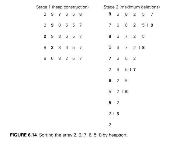
in Figure 6.11 is intentionally used so that you can compare the tree and array implementations of the bottom-up heap construction algorithm.)

Since we already know that the heap construction stage of the algorithm is in O(n), we have to investigate just the time efficiency of the second stage. For the number of key comparisons, C(n), needed for eliminating the root keys from the heaps of diminishing sizes from n to 2, we get the following inequality:

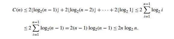
This means that C(n) ∈ O(n log n) for the second stage of heapsort. For both stages, we get O(n) + O(n log n) = O(n log n). A more detailed analysis shows that the time efficiency of heapsort is, in fact, in  (n log n) in both the worst and average cases. Thus, heapsort’s time efficiency falls in the same class as that of mergesort. Unlike the latter, heapsort is in-place, i.e., it does not require any extra storage. Timing experiments on random files show that heapsort runs more slowly than quicksort but can be competitive with mergesort.

Exercises 6.4

            a.  Construct a heap for the list 1, 8, 6, 5, 3, 7, 4 by the bottom-up algorithm.

            Construct a heap for the list 1, 8, 6, 5, 3, 7, 4 by successive key insertions (top-down algorithm).

            Is it always true that the bottom-up and top-down algorithms yield the same heap for the same input?

            Outline an algorithm for checking whether an array H [1..n] is a heap and determine its time efficiency.

            a. Find the smallest and the largest number of keys that a heap of height h can contain.

            Prove that the height of a heap with n nodes is equal to  log₂ n .

            Prove the following equality used in Section 6.4:

            a. Design an efficient algorithm for finding and deleting an element of the smallest value in a heap and determine its time efficiency.

            Design an efficient algorithm for finding and deleting an element of a given value v in a heap H and determine its time efficiency.

            Indicate the time efficiency classes of the three main operations of the priority queue implemented as

            an unsorted array.

            a sorted array.

            a binary search tree.

            an AVL tree.

            a heap.

            Sort the following lists by heapsort by using the array representation of heaps.

            1, 2, 3, 4, 5 (in increasing order)

            5, 4, 3, 2, 1 (in increasing order)

            S, O, R, T, I, N, G (in alphabetical order)

            Is heapsort a stable sorting algorithm?

            What variety of the transform-and-conquer technique does heapsort repre-sent?

            Which sorting algorithm other than heapsort uses a priority queue?

Implement three advanced sorting algorithms—mergesort, quicksort, and heapsort—in the language of your choice and investigate their performance on arrays of sizes n = 10³, 10⁴, 10⁵, and 10⁶. For each of these sizes consider

            randomly generated files of integers in the range [1..n].

            increasing files of integers 1, 2, . . . , n.

            decreasing files of integers n, n − 1, . . . , 1.

            Spaghetti sort Imagine a handful of uncooked spaghetti, individual rods whose lengths represent numbers that need to be sorted.

            Outline a “spaghetti sort”—a sorting algorithm that takes advantage of this unorthodox representation.

            What does this example of computer science folklore (see [Dew93]) have to do with the topic of this chapter in general and heapsort in particular?