Multiple Tasks and Multiple Processes

MULTIPLE TASKS AND MULTIPLE PROCESSES:

Tasks and Processes

Many (if not most) embedded computing systems do more than one thing that is, the environment can cause mode changes that in turn cause the embedded system to behave quite differently. For example, when designing a telephone answering machine,

We can define recording a phone call and operating the user’s control panel as distinct tasks, because they perform logically distinct operations and they must be performed at very different rates. These different tasks are part of the system’s functionality, but that application-level organization of functionality is often reflected in the structure of the program as well.

A process is a single execution of a program. If we run the same program two different times, we have created two different processes. Each process has its own state that includes not only its registers but all of its memory. In some OSs, the memory management unit is used to keep each process in a separate address space. In others, particularly lightweight RTOSs, the processes run in the same address space. Processes that share the same address space are often called threads.

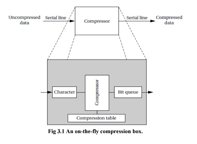
As shown in Figure 3.1, this device is connected to serial ports on both ends. The input to the box is an uncompressed stream of bytes. The box emits a compressed string of bits on the output serial line, based on a predefined compression table. Such a box may be used, for example, to compress data being sent to a modem.

The program’s need to receive and send data at different rates for example, the program may emit 2 bits for the first byte and then 7 bits for the second byte will obviously find itself reflected in the structure of the code. It is easy to create irregular, ungainly code to solve this problem; a more elegant solution is to create a queue of output bits, with those bits being removed from the queue and sent to the serial port in 8-bit sets.

But beyond the need to create a clean data structure that simplifies the control structure of the code, we must also ensure that we process the inputs and outputs at the proper rates. For example, if we spend too much time in packaging and emitting output characters, we may drop an input character. Solving timing problems is a more challenging problem.

The text compression box provides a simple example of rate control problems. A control panel on a machine provides an example of a different type of rate control problem, the asynchronous input.

The control panel of the compression box may, for example, include a compression mode button that disables or enables compression, so that the input text is passed through unchanged when compression is disabled. We certainly do not know when the user will push the compression mode button the button may be depressed asynchronously relative to the arrival of characters for compression.

Multirate Systems

Implementing code that satisfies timing requirements is even more complex when multiple rates of computation must be handled. Multirate embedded computing systems are very common, including automobile engines, printers, and cell phones. In all these systems, certain operations must be executed periodically, and each operation is executed at its own rate.

Timing Requirements on Processes

Processes can have several different types of timing requirements imposed on them by the application. The timing requirements on a set of processes strongly influence the type of scheduling that is appropriate. A scheduling policy must define the timing requirements that it uses to determine whether a schedule is valid. Before studying scheduling proper, we outline the types of process timing requirements that are useful in embedded system design.

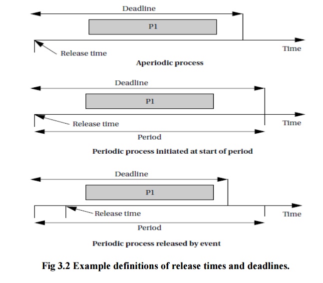
Figure 3.2 illustrates different ways in which we can define two important requirements on processes: release time and deadline.

The release time is the time at which the process becomes ready to execute; this is not necessarily the time at which it actually takes control of the CPU and starts to run. An aperiodic process is by definition initiated by an event, such as external data arriving or data computed by another process.

The release time is generally measured from that event, although the system may want to make the process ready at some interval after the event itself. For a periodically executed process, there are two common possibilities.

In simpler systems, the process may become ready at the beginning of the period. More sophisticated systems, such as those with data dependencies between processes, may set the release time at the arrival time of certain data, at a time after the start of the period.

A deadline specifies when a computation must be finished. The deadline for an aperiodic process is generally measured from the release time, since that is the only reasonable time reference. The deadline for a periodic process may in general occur at some time other than the end of the period.

Rate requirements are also fairly common. A rate requirement specifies how quickly processes must be initiated.

The period of a process is the time between successive executions. For example, the period of a digital filter is defined by the time interval between successive input samples.

The process’s rate is the inverse of its period. In a multirate system, each process executes at its own distinct rate.

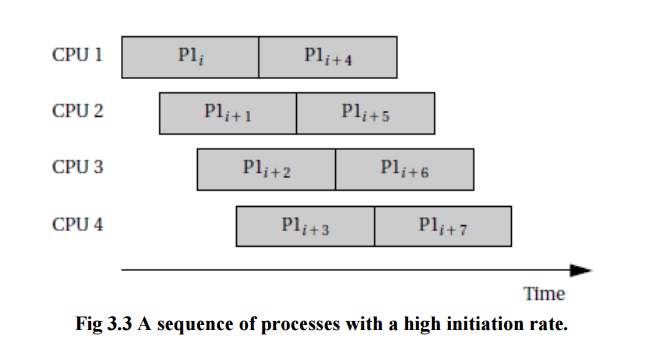
The most common case for periodic processes is for the initiation interval to be equal to the period. However, pipelined execution of processes allows the initiation interval to be less than the period. Figure 3.3 illustrates process execution in a system with four CPUs.

CPU Metrics

We also need some terminology to describe how the process actually executes. The initiation time is the time at which a process actually starts executing on the CPU. The completion time is the time at which the process finishes its work.

The most basic measure of work is the amount of CPU time expended by a process. The CPU time of process i is called Ci . Note that the CPU time is not equal to the completion time minus initiation time; several other processes may interrupt execution. The total CPU time consumed by a set of processes is

We need a basic measure of the efficiency with which we use the CPU. The simplest and most direct measure is utilization:

Utilization is the ratio of the CPU time that is being used for useful computations to the total available CPU time. This ratio ranges between 0 and 1, with 1 meaning that all of the available CPU time is being used for system purposes. The utilization is often expressed as a percentage. If we measure the total execution time of all processes over an interval of time t, then the CPU utilization is