Chapter: Principles of Compiler Design : Code optimization
Loops in Flow Graph
LOOPS IN FLOW GRAPH
A graph representation
of three-address statements, called a flow graph, is useful for understanding
code-generation algorithms, even if the graph is not explicitly constructed by
a code-generation algorithm. Nodes in the flow graph represent computations,
and the edges represent the flow of control.
Dominators:
In a flow graph, a node
d dominates node n, if every path from initial node of the flow graph to n goes
through d. This will be denoted by d dom n. Every initial node dominates all
the remaining nodes in the flow graph and the entry of a loop dominates all
nodes in the loop. Similarly every node dominates itself.
Example:
*In the flow graph below,
*Initial node,node1
dominates every node. *node 2 dominates itself
*node 3 dominates all
but 1 and 2. *node 4 dominates all but 1,2 and 3.
*node 5 and 6 dominates
only themselves,since flow of control can skip around either by goin through
the other.
*node 7 dominates 7,8
,9 and 10. *node 8 dominates 8,9 and 10.
*node 9 and 10 dominates only themselves.
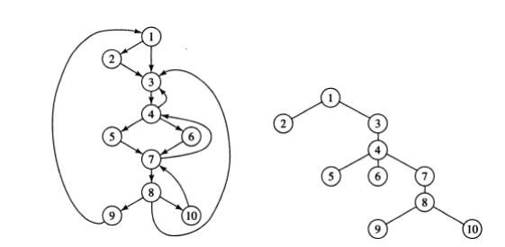
Fig.
5.3(a) Flow graph (b) Dominator tree
The way of presenting dominator information is in a
tree, called the dominator tree, in which
•
The initial node is the root.
•
The parent of each other node is its
immediate dominator.
•
Each node d dominates only its
descendents in the tree.
The existence of
dominator tree follows from a property of dominators; each node has a unique
immediate dominator in that is the last dominator of n on any path from the
initial node to n. In terms of the dom relation, the immediate dominator m has
the property is d=!n and d dom n, then d dom m.
***
D(1)={1}
D(2)={1,2}
D(3)={1,3}
D(4)={1,3,4}
D(5)={1,3,4,5}
D(6)={1,3,4,6}
D(7)={1,3,4,7}
D(8)={1,3,4,7,8}
D(9)={1,3,4,7,8,9}
D(10)={1,3,4,7,8,10}
Natural Loops:
One application of
dominator information is in determining the loops of a flow graph suitable for
improvement. There are two essential properties of loops:
Ø
A loop must have a single entrypoint,
called the header. This entry point-dominates all nodes in the loop, or it
would not be the sole entry to the loop.
Ø
There must be at least one way to
iterate the loop(i.e.)at least one path back to the headerOne way to find all
the loops in a flow graph is to search for edges in the flow graph whose heads
dominate their tails. If a→b is an edge, b is the head and a is the tail. These
types of
edges are called as back edges.
Example:
In the above graph,
7→4 4 DOM 7
10 →7 7 DOM 10
4→3
8→3
9 →1
The above edges will
form loop in flow graph. Given a back edge n → d, we define the natural loop of
the edge to be d plus the set of nodes that can reach n without going through
d. Node d is the header of the loop.
Algorithm: Constructing the natural loop
of a back edge.
Input: A flow graph G and a back edge n→d.
Output: The set loop consisting of all nodes in the
natural loop n→d.
Method: Beginning with
node n, we consider each node m*d that we know is in loop, to make sure that
m’s predecessors are also placed in loop. Each node in loop, except for d, is
placed once
on stack, so its
predecessors will be examined. Note that because d is put in the loop
initially, we never examine its predecessors, and thus find only those nodes
that reach n without going through d.
Procedure insert(m);
if m is not in loop then begin loop :=
loop U {m};
push m onto stack end;
stack : = empty;
loop : = {d};
insert(n);
while stack is not empty do begin
pop m, the first element of stack, off stack;
for
each predecessor p of m do insert(p)
end
Inner loops:
If we use the natural
loops as “the loops”, then we have the useful property that unless two loops
have the same header, they are either disjointed or one is entirely contained
in the
other. Thus, neglecting
loops with the same header for the moment, we have a natural notion of inner
loop: one that contains no other loop.
When two natural loops
have the same header, but neither is nested within the other, they are combined
and treated as a single loop.
Pre-Headers:
Several transformations
require us to move statements “before the header”. Therefore begin treatment of
a loop L by creating a new block, called the preheader. The pre-header has only
the header as successor, and all edges which formerly entered the header of L
from outside L instead enter the pre-header. Edges from inside loop L to the
header are not changed. Initially the pre-header is empty, but transformations
on L may place statements in it.
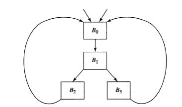
Fig.
5.4 Two loops with the same header
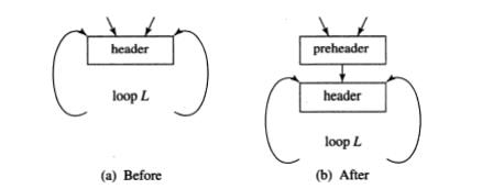
Fig. 5.5
Introduction of the preheader
Reducible flow graphs:
Reducible flow graphs
are special flow graphs, for which several code optimization transformations
are especially easy to perform, loops are unambiguously defined, dominators can
be easily calculated, data flow analysis problems can also be solved
efficiently. Exclusive use of structured flow-of-control statements such as
if-then-else, while-do, continue, and break statements produces programs whose
flow graphs are always reducible.
The most important properties of reducible flow
graphs are that
1.
There are no umps into the middle of
loops from outside;
2.
The only entry to a loop is through its
header
Definition:
A flow graph G is
reducible if and only if we can partition the edges into two disjoint groups,
forward edges and back edges, with the following properties.
1.
The forward edges from an acyclic graph
in which every node can be reached from initial node of G.
2.
The back edges consist only of edges
where heads dominate theirs tails.
Example: The above flow
graph is reducible. If we know the relation DOM for a flow graph, we can find
and remove all the back edges. The remaining edges are forward edges. If the
forward edges form an acyclic graph, then we can say the flow graph reducible.
In the above example remove the five back edges 4→3, 7→4, 8→3, 9→1 and 10→7
whose heads dominate their tails, the remaining graph is acyclic.
Related Topics