Chapter: Principles of Compiler Design : Code optimization
Introduction to Global Dataflow Analysis
INTRODUCTION TO GLOBAL DATAFLOW ANALYSIS
In order to do code optimization and a good job of code generation , compiler needs to collect information about the program as a whole and to distribute this information to each block in the flow graph. A compiler could take advantage of “reaching definitions” , such as knowing
where a variable like
debug was last defined before reaching a given block, in order to perform
transformations are just a few examples of data-flow information that an
optimizing compiler collects by a process known as data-flow analysis.
Data-flow information
can be collected by setting up and solving systems of equations of the form :
out
[S] = gen [S] U ( in [S] - kill [S] )
This equation can be read as “ the information at
the end of a statement is either generated within the statement , or enters at
the beginning and is not killed as control flows through the statement.” Such
equations are called data-flow equation.
1.
The details of how data-flow equations
are set and solved depend on three factors. The notions of generating and
killing depend on the desired information, i.e., on the data flow analysis
problem to be solved. Moreover, for some problems, instead of proceeding along
with flow of control and defining out[S] in terms of in[S], we need to proceed
backwards and define in[S] in terms of out[S].
2.
Since data flows along control paths,
data-flow analysis is affected by the constructs in a program. In fact, when we
write out[s] we implicitly assume that there is unique end point where control
leaves the statement; in general, equations are set up at the level of basic
blocks rather than statements, because blocks do have unique end points.
3.
There are subtleties that go along with
such statements as procedure calls, assignments through pointer variables, and
even assignments to array variables.
Points and Paths:
Within a basic block,
we talk of the point between two adjacent statements, as well as the point
before the first statement and after the last. Thus, block B1 has four points:
one before any of the assignments and one after each of the three assignments.
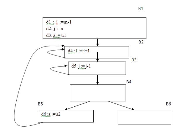
Fig.
5.6 A flow graph
Now let us take a
global view and consider all the points in all the blocks. A path from p1 to pn
is a sequence of points p1, p2,….,pn such that for each i between 1 and n-1,
either
1.
Pi is the point immediately preceding a
statement and pi+1 is the point immediately following that statement in the
same block, or
2.
Pi is the end of some block and pi+1 is
the beginning of a successor block.
Reaching definitions:
A definition of
variable x is a statement that assigns, or may assign, a value to x. The most
common forms of definition are assignments to x and statements that read a
value from an i/o device and store it in x. These statements certainly define a
value for x, and they are referred to as unambiguous definitions of x. There
are certain kinds of statements that may define a value for x; they are called
ambiguous definitions.
The most usual forms of ambiguous definitions of x
are:
1.
A call of a procedure with x as a
parameter or a procedure that can access x because x is in the scope of the
procedure.
2.
An assignment through a pointer that
could refer to x. For example, the assignment *q:=y is a definition of x if it
is possible that q points to x. we must assume that an assignment through a
pointer is a definition of every variable.
We say a definition d reaches a point p if there is a path from the point immediately following d to p, such that d is not “killed” along that path. Thus a point can be reached by an unambiguous definition and an ambiguous definition of the appearing later along one path.

Fig.
5.7 Some structured control constructs
Data-flow analysis of structured programs:
Flow graphs for control
flow constructs such as do-while statements have a useful property: there is a
single beginning point at which control enters and a single end point that
control leaves from when execution of the statement is over. We exploit this
property when we talk of the definitions reaching the beginning and the end of
statements with the following syntax.
S->id: = E| S; S | if E then S else S | do S
while E
E->id + id| id
Expressions in this
language are similar to those in the intermediate code, but the flow graphs for
statements have restricted forms.
We define a portion of
a flow graph called a region to be a set of nodes N that includes a header,
which dominates all other nodes in the region. All edges between nodes in N are
in the region, except for some that enter the header. The portion of flow graph
corresponding to a statement S is a region that obeys the further restriction
that control can flow to just one outside block when it leaves the region.
We say that the beginning
points of the dummy blocks at the statement’s region are the beginning and end
points, respective equations are inductive, or syntax-directed, definition of
the sets in[S], out[S], gen[S], and kill[S] for all statements S. gen[S] is the
set of definitions “generated” by S while kill[S] is the set of definitions
that never reach the end of S.
• Consider the following data-flow equations for
reaching definitions :
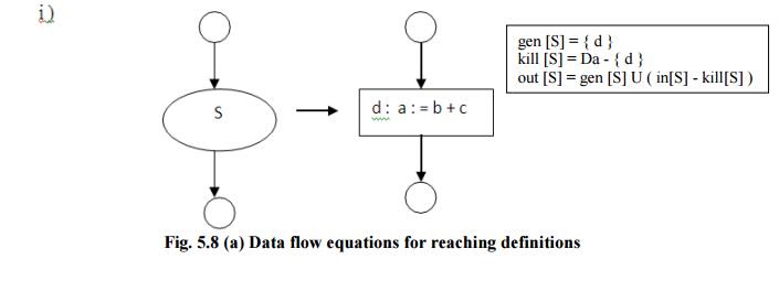
Fig.
5.8 (a) Data flow equations for reaching definitions
Observe the rules for a
single assignment of variable a. Surely that assignment is a definition of a,
say d. Thus
gen[S]={d}
On the other hand, d “kills” all other definitions
of a, so we write
Kill[S]
= Da - {d}
Where, Da is the set of all definitions in the
program for variable a.
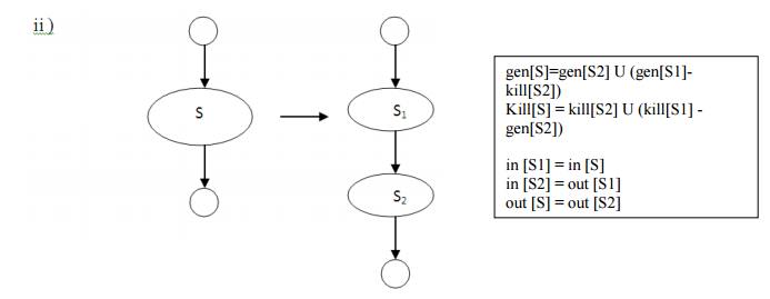
Fig.
5.8 (b) Data flow equations for reaching definitions
Under what
circumstances is definition d generated by S=S1; S2? First of all, if it is
generated by S2, then it is surely generated by S. if d is generated by S1, it
will reach the end of S provided it is not killed by S2. Thus, we write
gen[S]=gen[S2]
U (gen[S1]-kill[S2])
Similar reasoning applies to the killing of a
definition, so we have
Kill[S]
= kill[S2] U (kill[S1] - gen[S2])
Conservative estimation of data-flow
information:
There is a subtle
miscalculation in the rules for gen and kill. We have made the assumption that
the conditional expression E in the if and do statements are “uninterpreted”;
that
is, there exists inputs to the program that make
their branches go either way.
We
assume that any graph-theoretic path in the flow graph is also an execution
path, i.e., a path that is executed when the program is run with least one
possible input. When we compare the computed gen with the “true” gen we
discover that the true gen is always a subset of the computed gen. on the other
hand, the true kill is always a superset of the computed kill.
These containments hold
even after we consider the other rules. It is natural to wonder whether these
differences between the true and computed gen and kill sets present a serious
obstacle to data-flow analysis. The answer lies in the use intended for these
data.
Overestimating the set
of definitions reaching a point does not seem serious; it merely stops us from
doing an optimization that we could legitimately do. On the other hand,
underestimating the set of definitions is a fatal error; it could lead us into
making a change in the program that changes what the program computes. For the
case of reaching definitions, then, we call a set of definitions safe or
conservative if the estimate is a superset of the true set of reaching
definitions. We call the estimate unsafe, if it is not necessarily a superset
of the truth.
Returning now to the
implications of safety on the estimation of gen and kill for reaching
definitions, note that our discrepancies, supersets for gen and subsets for
kill are both in the safe direction. Intuitively, increasing gen adds to the
set of definitions that can reach a point, and cannot prevent a definition from
reaching a place that it truly reached. Decreasing kill can only increase the
set of definitions reaching any given point.
Computation of in and out:
Many data-flow problems
can be solved by synthesized translation to compute gen and kill. It can be used,
for example, to determine computations. However, there are other kinds of
data-flow information, such as the reaching-definitions problem. It turns out
that in is an inherited attribute, and out is a synthesized attribute depending
on in. we intend that in[S] be the set of definitions reaching the beginning of
S, taking into account the flow of control throughout the entire program,
including statements outside of S or within which S is nested.
The set out[S] is
defined similarly for the end of s. it is important to note the distinction
between out[S] and gen[S]. The latter is the set of definitions that reach the
end of S without following paths outside S. Assuming we know in[S] we compute
out by equation, that is
Out[S]
= gen[S] U (in[S] - kill[S])
Considering cascade of
two statements S1; S2, as in the second case. We start by observing in[S1]=in[S].
Then, we recursively compute out[S1], which gives us in[S2], since a definition
reaches the beginning of S2 if and only if it reaches the end of S1. Now we can
compute out[S2], and this set is equal to out[S].
Consider the
if-statement. we have conservatively assumed that control can follow either
branch, a definition reaches the beginning of S1 or S2 exactly when it reaches
the beginning of S. That is,
in[S1]
= in[S2] = in[S]
If a definition reaches
the end of S if and only if it reaches the end of one or both substatements;
i.e,
out[S]=out[S1]
U out[S2]
Representation of sets:
Sets of definitions,
such as gen[S] and kill[S], can be represented compactly using bit vectors. We
assign a number to each definition of interest in the flow graph. Then bit
vector representing a set of definitions will have 1 in position I if and only
if the definition numbered I is in the set.
The number of
definition statement can be taken as the index of statement in an array holding
pointers to statements. However, not all definitions may be of interest during
global data-flow analysis. Therefore the number of definitions of interest will
typically be recorded in a separate table.
A bit vector
representation for sets also allows set operations to be implemented
efficiently. The union and intersection of two sets can be implemented by
logical or and logical and, respectively, basic operations in most
systems-oriented programming languages. The difference A-B of sets A and B can
be implement complement of B and then using logical and to compute A
Local reaching definitions:
Space for data-flow
information can be traded for time, by saving information only at certain points
and, as needed, recomputing information at intervening points. Basic blocks are
usually treated as a unit during global flow analysis, with attention
restricted to only those points that are the beginnings of blocks.
Since there are usually
many more points than blocks, restricting our effort to blocks is a significant
savings. When needed, the reaching definitions for all points in a block can be
calculated from the reaching definitions for the beginning of a block.
Use-definition chains:
It is often convenient
to store the reaching definition information as” use-definition chains” or
“ud-chains”, which are lists, for each use of a variable, of all the
definitions that reaches that use. If a use of variable a in block B is
preceded by no unambiguous definition of a, then ud-chain for that use of a is
the set of definitions in in[B] that are definitions of a.in addition, if there
are ambiguous definitions of a ,then all of these for which no unambiguous
definition of a lies between it and the use of a are on the ud-chain for this
use of a.
Evaluation order:
The techniques for
conserving space during attribute evaluation, also apply to the computation of
data-flow information using specifications. Specifically, the only constraint
on the evaluation order for the gen, kill, in and out sets for statements is
that imposed by dependencies between these sets. Having chosen an evaluation
order, we are free to release the space for a set after all uses of it have
occurred. Earlier circular dependencies between attributes were not allowed,
but we have seen that data-flow equations may have circular dependencies.
General control flow:
Data-flow analysis must
take all control paths into account. If the control paths are evident from the
syntax, then data-flow equations can be set up and solved in a syntax directed
manner. When programs can contain goto statements or even the more disciplined
break and continue statements, the approach we have taken must be modified to
take the actual control paths into account.
Several approaches may be taken. The iterative method works arbitrary flow graphs. Since the flow graphs obtained in the presence of break and continue statements are reducible, such constraints can be handled systematically using the interval-based methods. However, the syntax-directed approach need not be abandoned when break and continue statements are allowed.
Related Topics