Properties, Limitations, Example Solved Problems - Karl PearsonŌĆÖs Correlation Coefficient | 12th Statistics : Chapter 4 : Correlation Analysis
Chapter: 12th Statistics : Chapter 4 : Correlation Analysis
Karl PearsonŌĆÖs Correlation Coefficient
KARL PEARSONŌĆÖS CORRELATION COEFFICIENT
When there exists some relationship between two measurable
variables, we compute the degree of relationship using the correlation
coefficient.
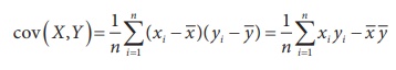
Co-variance
Let (X,Y) be a bivariable normal random variable where V(X)
and V(Y) exists. Then, covariance between X and Y
is defined as
cov(X,Y) = E[(X-E(X))(Y-E(Y))]
= E(XY) ŌĆō E(X)E(Y)
If (xi,yi), i=1,2, ...,
n is a set of n realisations of (X,Y), then the
sample covariance between
X and Y can
be calculated from
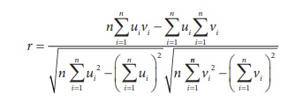
1. KarlŌĆéPearsonŌĆÖsŌĆécoefficientŌĆéofŌĆécorrelation
When X and Y are linearly related and (X,Y)
has a bivariate normal distribution, the co-efficient of correlation
between X and Y is defined as
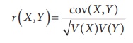
This is also called as product moment correlation co-efficient
which was defined by Karl Pearson.
Based on a given set of n paired observations (xi,yi),
i=1,2, ... n the sample correlation co-efficient between X and
Y can be calculated from
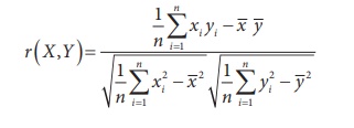
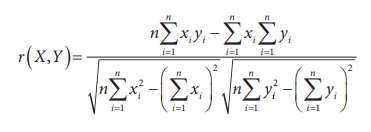
or, equivalently
2. Properties
1. The correlation coefficient between X
and Y is same as the correlation coefficient between Y and X (i.e,
rxy = ryx ).
2. The correlation coefficient is free from the
units of measurements of X and Y
3. The correlation coefficient is unaffected by change of scale
and origin.
Thus, if ui = [xi
ŌĆō A] /c and vi = [yi
ŌĆō B] /d with c ŌēĀ 0 and d ŌēĀ 0 i=1,2, ..., n
where A and B are arbitrary values.
Remark 1: If the widths between the values of the variabls are not equal
then take c = 1 and d = 1.
Interpretation
The correlation coefficient lies between -1 and +1. i.e. -1
Ōēż r Ōēż 1
┬Ę
A positive value of ŌĆśrŌĆÖ indicates positive correlation.
┬Ę
A negative value of ŌĆśrŌĆÖ indicates negative correlation
┬Ę
If r = +1, then the correlation is perfect positive
┬Ę
If r = ŌĆō1, then the correlation is perfect negative.
┬Ę
If r = 0, then the variables are uncorrelated.
┬Ę
If r Ōēź
0.7 then the correlation will be of higher degree. In interpretation we use the
adjective ŌĆśhighlyŌĆÖ
┬Ę
If X and Y are independent, then rxy
= 0. However the converse need not be true.
Example 4.1
The following data gives the heights(in inches) of father and his
eldest son. Compute the correlation coefficient between the heights of fathers
and sons using Karl PearsonŌĆÖs method.
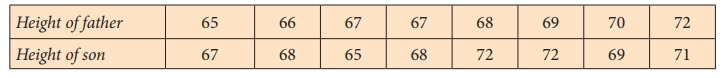
Solution:
Let x denote height of father and y denote height of
son. The data is on the ratio scale.
We use Karl PearsonŌĆÖs method.
Calculation
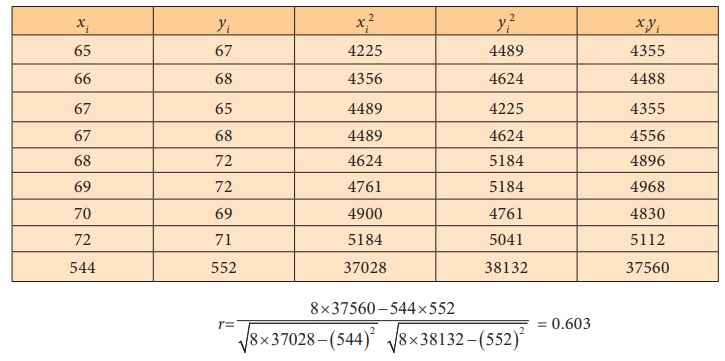
Heights of father and son are positively correlated. It means that
on the average , if fathers are tall then sons will probably tall and if
fathers are short, probably sons may be short.
Short-cut method
Let A = 68 , B = 69, c = 1 and d = 1
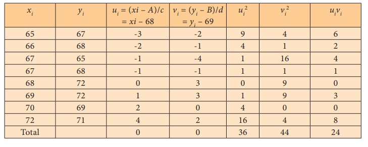
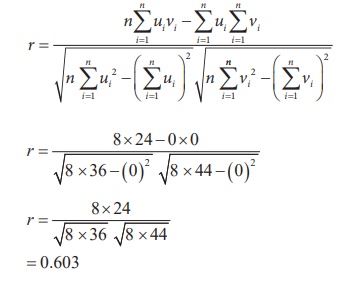
Note: The correlation coefficient computed by using direct method
and short-cut method is the same.
Example 4.2
The following are the marks scored by 7 students in two tests in a
subject. Calculate coefficient of correlation from the following data and
interpret.
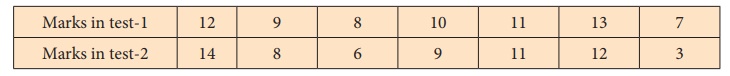
Solution:
Let x denote marks in test-1 and y denote marks in
test-2.
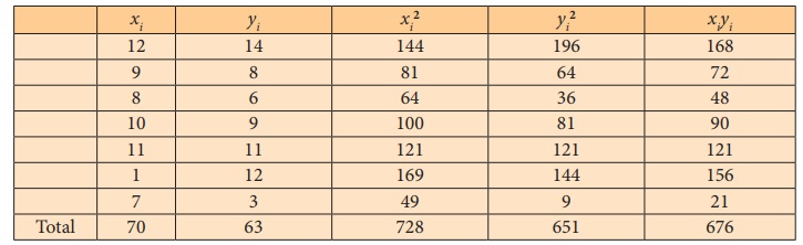

There is a high positive correlation between test -1 and test-2.
That is those who perform well in test-1 will also perform well in test-2 and
those who perform poor in test-1 will perform poor in test- 2.
The students can also verify the results by using shortcut method.
3. Limitations of Correlation
Although correlation is a powerful tool, there are some limitations in using it:
1. Outliers (extreme observations) strongly influence the correlation coefficient. If we see outliers in our data, we should be careful about the conclusions we draw from the value of r. The outliers may be dropped before the calculation for meaningful conclusion.
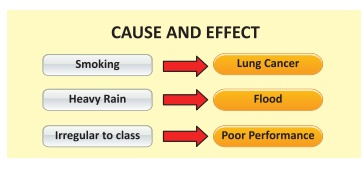
2. Correlation does not imply causal relationship. That a change
in one variable causes a change in another.
NOTE
1. Uncorrelated : Uncorrelated (r
= 0) implies no ŌĆślinear relationshipŌĆÖ. But there may exist non-linear
relationship (curvilinear relationship).
Example: Age and health care are related. Children and elderly people
need much more health care than middle aged persons as seen from the
following graph.
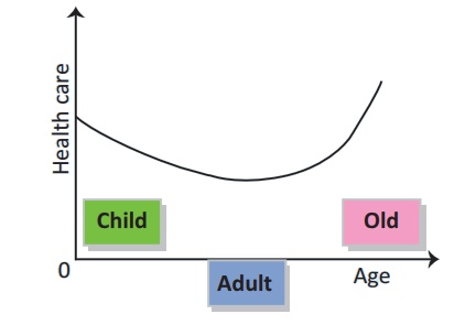
However, if we compute the linear correlation r for such
data, it may be zero implying age and health care are uncorrelated, but
non-linear correlation is present.
2. Spurious Correlation : The word ŌĆśspuriousŌĆÖ from Latin means ŌĆśfalseŌĆÖ or ŌĆśillegitimateŌĆÖ. Spurious correlation means an association extracted from correlation coefficient that may not exist in reality.
Related Topics