Functions - Mathematical Methods for Economics

Functions

1. Definition

A function is a mathematical relationship in which the values of a dependent variable are determined by the values of one or more independent variables.

Functions with a single independent variable are called Simple Univariate functions. There is a one to one correspondence. Functions,with more than one independent variable, are called Multivariate functions. The independent variable is often designated by X. The dependent variable is often designated by Y. For example, Y is function of X which means Y depends on X or the value of Y is determined by the value of X. Mathematically one can write Y = f(X).

2. Linear Equation

A statement of relationship between two quantities is called an equation. In an equation, if the largest power of the independent variable is one, then it is called as Linear Equation. Such equations when graphed give straight lines. For example Y = 100-10X.

For a straight line, there are two variables namely X and Y. X is called independent variable and Y is called dependent variable.

When ‘X’ value increases by one unit, then the corresponding change in the ‘Y’ value is called as the slope of the line. Slope of the line is obtained by the formula,

m = slope (marginal change)

Where (X₁, Y₁) and (X₂, Y₂) are two arbitrary points

Slope or Gradient of the line represents the ratio of the changes in vertical and horizontal lines.

The formula for constructing a straight line is

(Y - Y₁) = m (X - X₁)

If the two points are (0, 0) and (X, Y) then the formula is Y = Mx

Example 12.1

Find the equation of a straight line which passes through two points (2, 2) and (4, -8) which are (X₁, Y₁) and (X₂, Y₂) respectively.

Note: For drawing a straight line, at least two points are required. Many straight lines can pass through a single point.

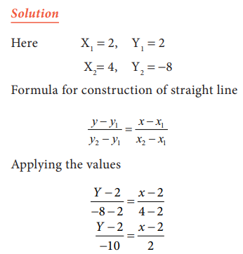
2(y-2) = -10(x-2)

2y-4 = -10x +20

2y = -10x+24

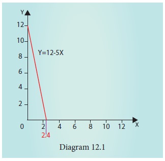
y=-5x +12

-5 is slope, denoted by m

12 is y intercept, or constantdenoted by c This is of the form Y = mX + c

y = 12-5x when x = 0; y = 12 

When y = 0; x = 12/5 = 2.4 (This line looks likes demand line in micro economics )

3. Application in Economics

By applying the above method, the demand and supply functions are obtained.

Demand Function: Q_d = f (P_x ) where Q_d stands for Quantity demand of a commodity and P_x is the price of that commodity.

Supply Function: Qs = f (P_x) where ‘Q_s’ stands for Quantity supplied of a commodity and Px is the price of that commodity.

In the example 12.1 the equation Y -5X + 12 has been obtained. It is a linear function.

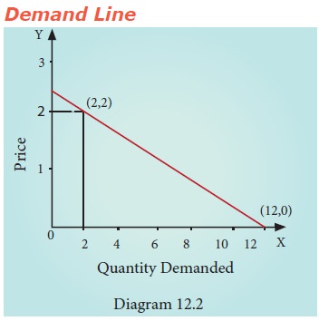
Since slope is negative here, this function could be a demand function.

Price-quantity relationship is negative in demand function.

Q_d = 12-5 X  or Qd = 12-5P. If P = 2, Qd = 2.

When P assumes 0, only 12 alone remains in the equation. This is called Intercept or Constant, if P = 0 and Qd = 12.

In Marshallian analysis, money terms measured in Y-axis and physical units are measured in X-axis. Accordingly, price is measured in Y-axis and quantity demanded is measured in X-axis

Example: 12.2

Find the supply function of a commodity such that the quantity supplied is zero, when the price is  Rs.5 or below and the supply (quantity) increases continuously at the constant rate of 10 units for each one rupee rise when the price is above  Rs.5.

Solution:

To construct the linear supply function atleast two points are needed. First data point of supply function is obtained from the statement that the quantity supplied is zero, when the price is  Rs.5, that is (0, 5). The second and third data points of supply function can be obtained from the statement that supply increases 10 units for each one rupee rise in price, that is (10, 6) & (20, 7).

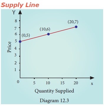
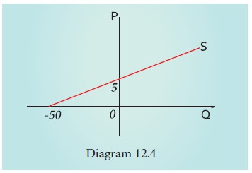
When p = 5, supply is zero. When p = 6, supply is 10 and so on. When p is less than 5, say 4, supply is -10, which is possible in mathematics. But it is meaningless in Economics. Normally supply curve originates from zero, noting that when price is zero, supply is also zero.

The equation of the straight line joining two data points (10, 6) and (20, 7) is given as The equation of the straight line is

substituting the values of (x1, y1) (x2, y2) by (10, 6) , (20, 7) respectively,

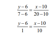
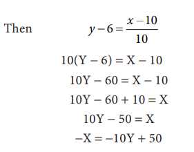
10(Y - 6) = X - 10

10Y - 60 = X - 10

10Y - 60 + 10 = X

10Y - 50 = X

-X = -10Y + 50

Multiplying both sides by minus (-), we get

X = -50 + 10Y

Considering X as quantity supplied and Y as price (p)

Then X = 10p - 50 (or)

X = -50 + 10 p

If Price = 0; Q = -50

If Q = 0; P = 5

Note: The coefficient of ‘p’ is - in demand function. Note: The coefficient of ‘p’ is - in demand function.

The coefficient of ‘p’ is + in supply function.

4. Equilibrium

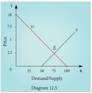
The point of intersection of demand line and supply line is known as equilibrium. The point of equilibrium is obtained by using the method of solving a set of equations. One can obtain the values of two unknowns with two equations. At equilibrium point,

Demand = Supply

(These are hypothetical examples)

100-10p = 50 + 10 p

100-50 = 20p

50 = 20p

p = 2.5

When p = 2.5, Demand = 100-10 (2.5) = 75

When P = 2.5, Supply = 50 +10 (2.5) = 75

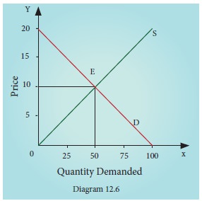
Example: 12.3

Find the equilibrium price and quantity by using the following demand and supply functions Qd = 100-5P and Qs = 5P respectively.

Solution:

Equilibrium is attained when,

Qs = Qd

5 P = 100 - 5 P

10P = 100

P = 10

When P = 10

In supply function

Qs = 5 P = 5 x 10 = 50

In demand function,

Qd = 100 - 5 P = 100 - 5(10) = 50

Hence at

P = 10, Qd = 50, Qs = 50.

Quantity demanded is equal to supply at 50 units when price is  Rs.10

Example: 12.4

The market demand curve is given by D = 50 - 5P. Find the maximum price beyond which nobody will buy the commodity.

Solution:

Given

Qd = 50 - 5P

5P = 50 - Qd

5P = 50 when Qd is zero.

P=50/5

P = 10 When P = 10, Demand is 0

Hence P = 10, which is the maximum price beyond which nobody will demand the commodity.

Example: 12.5

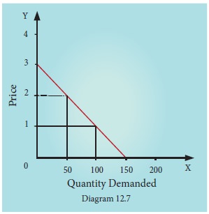
The demand for milk is given by

Find the linear demand function and its slope.

Solution:

Equation of demand function joining two data points (100, 1) and (50, 2) are (x1, y1) and (x2, y2) respectively.

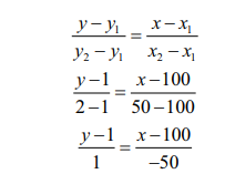
-50 (y - 1) = 1 (x - 100)

-50y + 50 = x - 100

-50y + 50 + 100 = x

-50y + 150 = x

x = 150 - 50y

Hence the demand function is

Qd = 150 – 50P and Slope m = – 50

Think and Do for Water Management in your area

Try to find the demand function for water in your street and the daily total demand for water in litre for all purposes.