Correlation

Correlation

Introduction

In the previous Chapter we have studied the characteristics of only one variable; example, marks, weights, heights, rainfalls, prices, ages, sales, etc. This type of analysis is called univariate analysis. Sometimes we may be interested to find if there is any relationship between the two variables under study. For example, the price of the commodity and its sale, height of a father and height of his son, price and demand, yield and rainfall, height and weight and so on. Thus the association of any two variables is known as correlation.

Correlation is the statistical analysis which measures and analyses the degree or extent to which two variables fluctuate with reference to each other.

1. Meaning of Correlation

The term correlation refers to the degree of relationship between two or more variables. If a change in one variable effects a change in the other variable, the variables are said to be correlated.

2. Types of correlation

Correlation is classified into many types, but the important are:

(i) Positive

(ii) Negative

Positive and negative correlation depends upon the direction of change of the variables.

Positive Correlation

If two variables tend to move together in the same direction that is, an increase in the value of one variable is accompanied by an increase in the value of the other variable; or a decrease in the value of one variable is accompanied by a decrease in the value of the other variable, then the correlation is called positive or direct correlation.

Example

(i) The heights and weights of individuals

(ii) Price and Supply

(iii) Rainfall and Yield of crops

(iv) The income and expenditure

Negative Correlation

If two variables tend to move together in opposite direction so that an increase or decrease in the values of one variable is accompanied by a decrease or increase in the value of the other variable, then the correlation is called negative or inverse correlation.

Example

(i) Price and demand

(ii) Repayment period and EMI

(iii) Yield of crops and price

No Correlation

Two variables are said to be uncorrelated if the change in the value of one variable has no connection with the change in the value of the other variable.

For example

We should expect zero correlation (no correlation) between weight of a person and the colour of his hair or the height of a person and the colour of his hair.

Simple correlation

The correlation between two variables is called simple correlation. The correlation in the case of more than two variables is called multiple correlation.

The following are the mathematical methods of correlation coefficient

(i) Scatter diagram

(ii) Karl Pearson’s Coefficient of Correlation

3. Scatter Diagram

Let (X₁ , Y₁),(X₂, Y₂) … (X _N , Y_N) be the N pairs of observation of the variables X and Y. If we plot the values of X along x - axis and the corresponding values of Y along y-axis, the diagram so obtained is called a scatter diagram. It gives us an idea of relationship between X and Y. The type of scatter diagram under a simple linear correlation is given below.

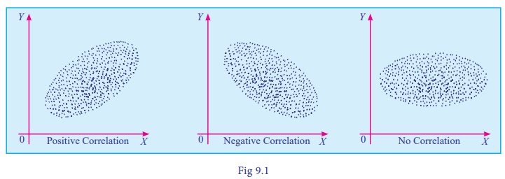
(i) If the plotted points show an upward trend, the correlation will be positive.

(ii) If the plotted points show a downward trend, the correlation will be negative.

(iii) If the plotted points show no trend the variables are said to be uncorrelated.

4. Karl Pearson’s Correlation Coefficient

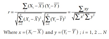
Karl Pearson, a great biometrician and statistician, suggested a mathematical method for measuring the magnitude of linear relationship between two variables say X and Y. Karl Pearson’s method is the most widely used method in practice and is known as Pearsonian Coefficient of Correlation. It is denoted by the symbol ‘r’ and defined as

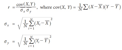
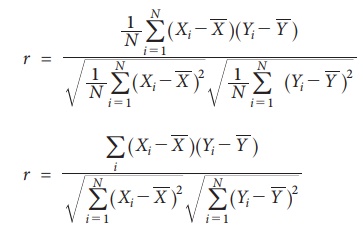
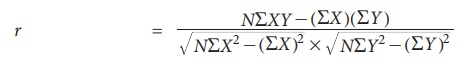
Hence the formula to compute Karl Pearson Correlation coefficient is

Interpretation of Correlation coefficient:

Coefficient of correlation lies between –1 and +1. Symbolically, –1≤ r ≤ + 1

·        When r =+1 , then there is perfect positive correlation between the variables.

·        When r=–1 , then there is perfect negative correlation between the variables.

·        When r=0, then there is no relationship between the variables, that is the variables are uncorrelated.

Thus, the coefficient of correlation describes the magnitude and direction of correlation.

Methods of computing Correlation Coefficient

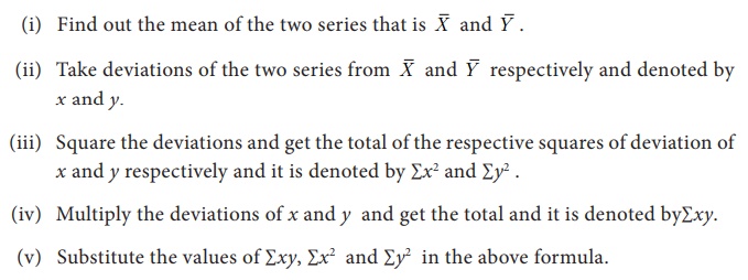
(i) When deviations are taken from Mean

Of all the several mathematical methods of measuring correlation, the Karl Pearson’s method, popularly known as Pearsonian coefficient of correlation, is most widely used in practice.

This method is to be applied only when the deviations of items are taken from actual means.

Steps to solve the problems:

Example 9.1

Calculate Karl Pearson’s coefficient of correlation from the following data:

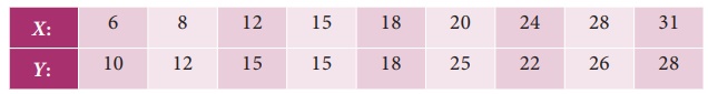
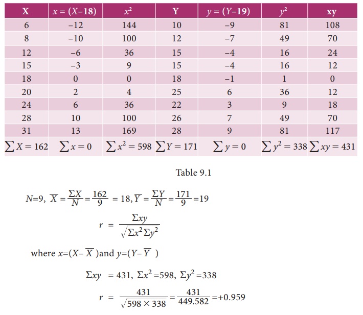
Solution:

(ii) When actual values are taken (without deviation)

when the values of X and Y are considerably small in magnitude the following formula can be used

Example 9.2

Calculate coefficient of correlation from the following data

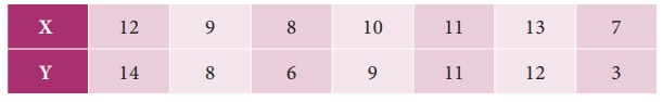
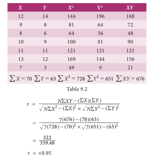
Solution:

In both the series items are in small number. Therefore correlation coefficient can also be calculated without taking deviations from actual means or assumed mean.

(iii) When deviations are taken from an Assumed mean

When actual means are in fractions, say the actual means of X and Y series are 20.167 and 29.23, the calculation of correlation by the method discussed above would involve too many calculations and would take a lot of time. In such cases we make use of the assumed mean method for finding out correlation. When deviations are taken from an assumed mean the following formula is applicable:

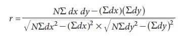
Where dx = X–A and dy=Y–B . Here A and B are assumed mean

NOTE

While applying assumed mean method, any value can be taken as the assumed mean and the answer will be the same. However, the nearer the assumed mean to the actual mean, the lesser will be the calculations.

Steps to solve the problems:

(i) Take the deviations of X series from an assumed mean, denote these deviations by dx and obtain the total that is Rdx .

(ii) Take the deviations of Y series from an assumed mean, denote these deviations by dy and obtain the total that is Rdy .

(iii) Square  dx and obtain the total Rdx² .

(iv) Square dy and obtain the total Rdy² .

(v) Multiply dx and dy and obtain the total Rdx dy

(vi)    Substitute the values of R dxdy , R dx, R dy, R dx2 and R dy2 in the formula given above.

Example 9.3

Find out the coefficient of correlation in the following case and interpret.

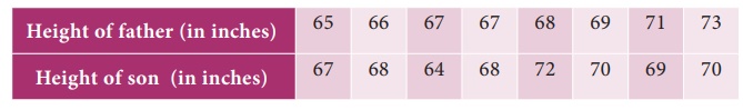
Solution:

Let us consider Height of father (in inches) is represented as X and Height of son (in inches) is represented as Y

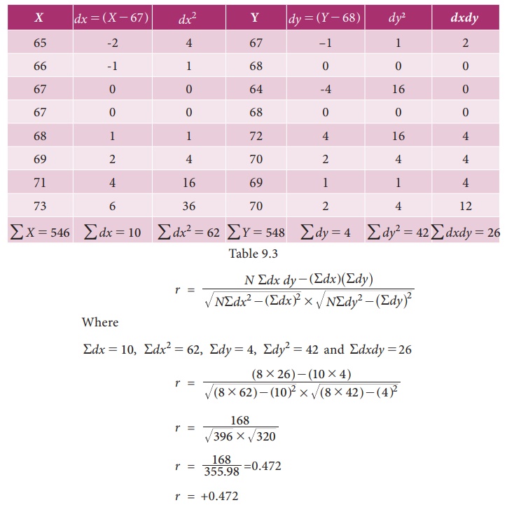
Heights of fathers and their respective sons are positively correlated.

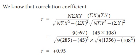
Example 9.4

Calculate the correlation coefficient from the following data

Solution

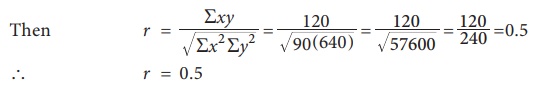
Example 9.5

From the following data calculate the correlation coefficient Rxy =120, Rx² =90, Ry² =640

Solution:

Given Rxy =120, Rx² =90, Ry² =640