Branch-and-Bound

Branch-and-Bound

Recall that the central idea of backtracking, discussed in the previous section, is to cut off a branch of the problem’s state-space tree as soon as we can deduce that it cannot lead to a solution. This idea can be strengthened further if we deal with an optimization problem. An optimization problem seeks to minimize or maximize some objective function (a tour length, the value of items selected, the cost of an assignment, and the like), usually subject to some constraints. Note that in the standard terminology of optimization problems, a feasible solution is a point in the problem’s search space that satisfies all the problem’s constraints (e.g., a Hamiltonian circuit in the traveling salesman problem or a subset of items whose total weight does not exceed the knapsack’s capacity in the knapsack problem), whereas an optimal solution is a feasible solution with the best value of the objective function (e.g., the shortest Hamiltonian circuit or the most valuable subset of items that fit the knapsack).

Compared to backtracking, branch-and-bound requires two additional items:

a way to provide, for every node of a state-space tree, a bound on the best value of the objective function1 on any solution that can be obtained by adding further components to the partially constructed solution represented by the node the value of the best solution seen so far

If this information is available, we can compare a node’s bound value with the value of the best solution seen so far. If the bound value is not better than the value of the best solution seen so far—i.e., not smaller for a minimization problem

and not larger for a maximization problem—the node is nonpromising and can be terminated (some people say the branch is “pruned”). Indeed, no solution obtained from it can yield a better solution than the one already available. This is the principal idea of the branch-and-bound technique.

In general, we terminate a search path at the current node in a state-space tree of a branch-and-bound algorithm for any one of the following three reasons:

The value of the node’s bound is not better than the value of the best solution seen so far.

The node represents no feasible solutions because the constraints of the problem are already violated.

The subset of feasible solutions represented by the node consists of a single point (and hence no further choices can be made)—in this case, we compare the value of the objective function for this feasible solution with that of the best solution seen so far and update the latter with the former if the new solution is better.

Assignment Problem

Let us illustrate the branch-and-bound approach by applying it to the problem of assigning n people to n jobs so that the total cost of the assignment is as small as possible. We introduced this problem in Section 3.4, where we solved it by exhaustive search. Recall that an instance of the assignment problem is specified by an n × n cost matrix C so that we can state the problem as follows: select one element in each row of the matrix so that no two selected elements are in the same column and their sum is the smallest possible. We will demonstrate how this problem can be solved using the branch-and-bound technique by considering the same small instance of the problem that we investigated in Section 3.4:

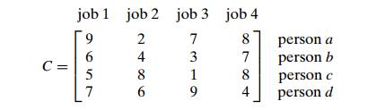
How can we find a lower bound on the cost of an optimal selection without actually solving the problem? We can do this by several methods. For example, it is clear that the cost of any solution, including an optimal one, cannot be smaller than the sum of the smallest elements in each of the matrix’s rows. For the instance here, this sum is 2 + 3 + 1 + 4 = 10. It is important to stress that this is not the cost of any legitimate selection (3 and 1 came from the same column of the matrix); it is just a lower bound on the cost of any legitimate selection. We can and will apply the same thinking to partially constructed solutions. For example, for any legitimate selection that selects 9 from the first row, the lower bound will be 9 + 3 + 1 + 4 = 17.

One more comment is in order before we embark on constructing the prob-lem’s state-space tree. It deals with the order in which the tree nodes will be generated. Rather than generating a single child of the last promising node as we did in backtracking, we will generate all the children of the most promising node among nonterminated leaves in the current tree. (Nonterminated, i.e., still promising, leaves are also called live.) How can we tell which of the nodes is most promising? We can do this by comparing the lower bounds of the live nodes. It is sensible to consider a node with the best bound as most promising, although this does not, of course, preclude the possibility that an optimal solution will ul-timately belong to a different branch of the state-space tree. This variation of the strategy is called the best-first branch-and-bound.

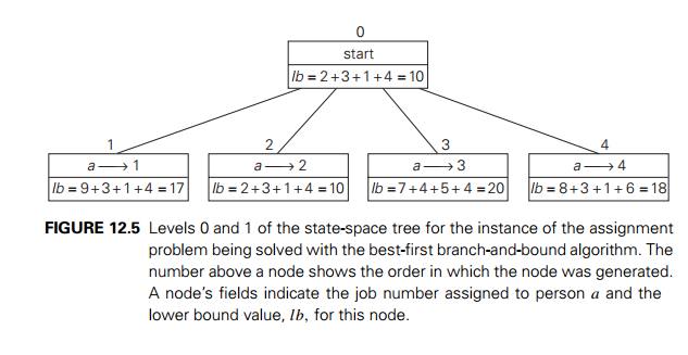
So, returning to the instance of the assignment problem given earlier, we start with the root that corresponds to no elements selected from the cost matrix. As we already discussed, the lower-bound value for the root, denoted lb, is 10. The nodes on the first level of the tree correspond to selections of an element in the first row of the matrix, i.e., a job for person a (Figure 12.5).

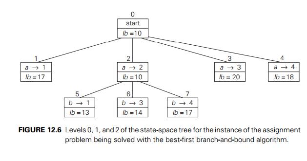
So we have four live leaves—nodes 1 through 4—that may contain an optimal solution. The most promising of them is node 2 because it has the smallest lower-bound value. Following our best-first search strategy, we branch out from that node first by considering the three different ways of selecting an element from the second row and not in the second column—the three different jobs that can be assigned to person b (Figure 12.6).

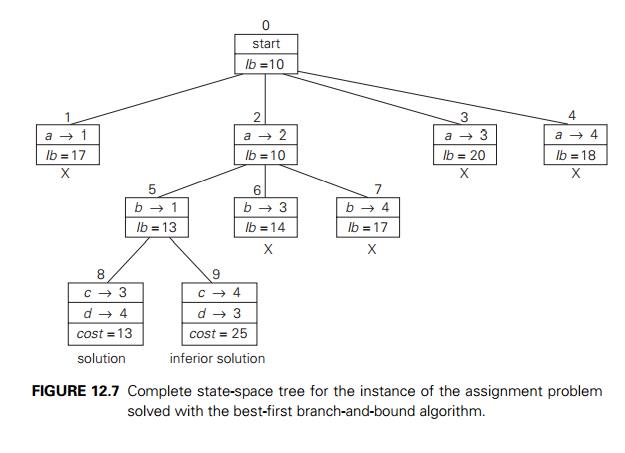
Of the six live leaves—nodes 1, 3, 4, 5, 6, and 7—that may contain an optimal solution, we again choose the one with the smallest lower bound, node 5. First, we consider selecting the third column’s element from c’s row (i.e., assigning person c to job 3); this leaves us with no choice but to select the element from the fourth column of d’s row (assigning person d to job 4). This yields leaf 8 (Figure 12.7), which corresponds to the feasible solution {a → 2, b → 1, c → 3, d → 4} with the total cost of 13. Its sibling, node 9, corresponds to the feasible solution {a → 2, b → 1, c → 4, d → 3} with the total cost of 25. Since its cost is larger than the cost of the solution represented by leaf 8, node 9 is simply terminated. (Of course, if

its cost were smaller than 13, we would have to replace the information about the best solution seen so far with the data provided by this node.)

Now, as we inspect each of the live leaves of the last state-space tree—nodes 1, 3, 4, 6, and 7 in Figure 12.7—we discover that their lower-bound values are not smaller than 13, the value of the best selection seen so far (leaf 8). Hence, we terminate all of them and recognize the solution represented by leaf 8 as the optimal solution to the problem.

Before we leave the assignment problem, we have to remind ourselves again that, unlike for our next examples, there is a polynomial-time algorithm for this problem called the Hungarian method (e.g., [Pap82]). In the light of this efficient algorithm, solving the assignment problem by branch-and-bound should be con-sidered a convenient educational device rather than a practical recommendation.

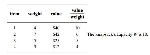
Knapsack Problem

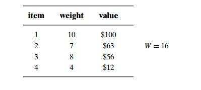
Let us now discuss how we can apply the branch-and-bound technique to solving the knapsack problem. This problem was introduced in Section 3.4: given n items of known weights w_i and values v_i, i = 1, 2, . . . , n, and a knapsack of capacity W , find the most valuable subset of the items that fit in the knapsack. It is convenient to order the items of a given instance in descending order by their value-to-weight ratios. Then the first item gives the best payoff per weight unit and the last one gives the worst payoff per weight unit, with ties resolved arbitrarily:

v₁/w₁ ≥ v₂/w₂ ≥ ^{. . .} ≥ v_n/w_n.

It is natural to structure the state-space tree for this problem as a binary tree constructed as follows (see Figure 12.8 for an example). Each node on the ith level of this tree, 0 ≤ i ≤ n, represents all the subsets of n items that include a particular selection made from the first i ordered items. This particular selection is uniquely determined by the path from the root to the node: a branch going to the left indicates the inclusion of the next item, and a branch going to the right indicates its exclusion. We record the total weight w and the total value v of this selection in the node, along with some upper bound ub on the value of any subset that can be obtained by adding zero or more items to this selection.

A simple way to compute the upper bound ub is to add to v, the total value of the items already selected, the product of the remaining capacity of the knapsack W − w and the best per unit payoff among the remaining items, which is v_i+1 /  w_i+1:

As a specific example, let us apply the branch-and-bound algorithm to the same instance of the knapsack problem we solved in Section 3.4 by exhaustive search. (We reorder the items in descending order of their value-to-weight ratios, though.)

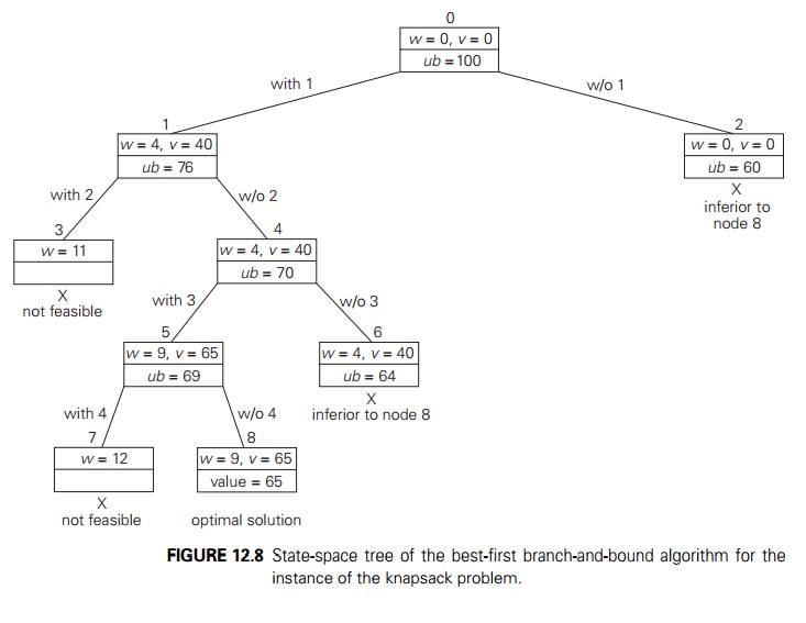
At the root of the state-space tree (see Figure 12.8), no items have been selected as yet. Hence, both the total weight of the items already selected w and their total value v are equal to 0. The value of the upper bound computed by formula (12.1) is $100. Node 1, the left child of the root, represents the subsets that include item 1. The total weight and value of the items already included are 4 and $40, respectively; the value of the upper bound is 40 + (10 − 4) ∗ 6 = $76. Node 2 represents the subsets that do not include item 1. Accordingly, w = 0, v = $0, and ub = 0 + (10 − 0) ∗ 6 = $60. Since node 1 has a larger upper bound than the upper bound of node 2, it is more promising for this maximization problem, and we branch from node 1 first. Its children—nodes 3 and 4—represent subsets with item 1 and with and without item 2, respectively. Since the total weight w of every subset represented by node 3 exceeds the knapsack’s capacity, node 3 can be terminated immediately. Node 4 has the same values of w and v as its parent; the upper bound ub is equal to 40 + (10 − 4) ∗ 5 = $70. Selecting node 4 over node 2 for the next branching (why?), we get nodes 5 and 6 by respectively including and excluding item 3. The total weights and values as well as the upper bounds for these nodes are computed in the same way as for the preceding nodes. Branching from node 5 yields node 7, which represents no feasible solutions, and node 8, which represents just a single subset {1, 3} of value $65. The remaining live nodes 2 and 6 have smaller upper-bound values than the value of the solution represented by node 8. Hence, both can be terminated making the subset {1, 3} of node 8 the optimal solution to the problem.

Solving the knapsack problem by a branch-and-bound algorithm has a rather unusual characteristic. Typically, internal nodes of a state-space tree do not define a point of the problem’s search space, because some of the solution’s components remain undefined. (See, for example, the branch-and-bound tree for the assign-ment problem discussed in the preceding subsection.) For the knapsack problem, however, every node of the tree represents a subset of the items given. We can use this fact to update the information about the best subset seen so far after generating each new node in the tree. If we had done this for the instance investi-gated above, we could have terminated nodes 2 and 6 before node 8 was generated because they both are inferior to the subset of value $65 of node 5.

Traveling Salesman Problem

We will be able to apply the branch-and-bound technique to instances of the traveling salesman problem if we come up with a reasonable lower bound on tour lengths. One very simple lower bound can be obtained by finding the smallest element in the intercity distance matrix D and multiplying it by the number of cities n. But there is a less obvious and more informative lower bound for instances with symmetric matrix D, which does not require a lot of work to compute. It is not difficult to show (Problem 8 in this section’s exercises) that we can compute a lower bound on the length l of any tour as follows. For each city i, 1 ≤ i ≤ n, find the sum s_i of the distances from city i to the two nearest cities; compute the sum s of these n numbers, divide the result by 2, and, if all the distances are integers, round up the result to the nearest integer:

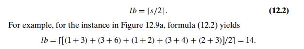
Moreover, for any subset of tours that must include particular edges of a given graph, we can modify lower bound (12.2) accordingly. For example, for all the Hamiltonian circuits of the graph in Figure 12.9a that must include edge (a, d), we get the following lower bound by summing up the lengths of the two shortest edges incident with each of the vertices, with the required inclusion of edges (a, d) and (d, a):

We now apply the branch-and-bound algorithm, with the bounding function given by formula (12.2), to find the shortest Hamiltonian circuit for the graph in

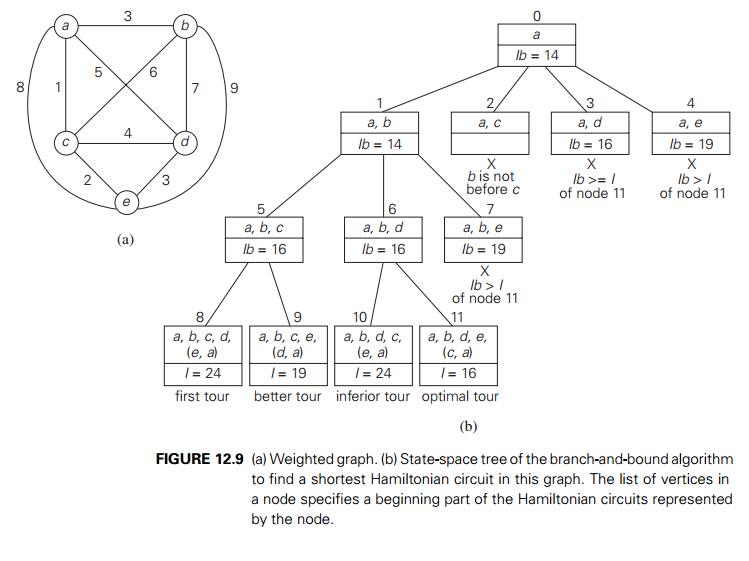
Figure 12.9a. To reduce the amount of potential work, we take advantage of two observations made in Section 3.4. First, without loss of generality, we can consider only tours that start at a. Second, because our graph is undirected, we can generate only tours in which b is visited before c. In addition, after visiting n − 1 = 4 cities, a tour has no choice but to visit the remaining unvisited city and return to the starting one. The state-space tree tracing the algorithm’s application is given in Figure 12.9b.

The comments we made at the end of the preceding section about the strengths and weaknesses of backtracking are applicable to branch-and-bound as well. To reiterate the main point: these state-space tree techniques enable us to solve many large instances of difficult combinatorial problems. As a rule, however, it is virtually impossible to predict which instances will be solvable in a realistic amount of time and which will not.

Incorporation of additional information, such as a symmetry of a game’s board, can widen the range of solvable instances. Along this line, a branch-and-bound algorithm can be sometimes accelerated by a knowledge of the objective function’s value of some nontrivial feasible solution. The information might be obtainable—say, by exploiting specifics of the data or even, for some problems, generated randomly—before we start developing a state-space tree. Then we can use such a solution immediately as the best one seen so far rather than waiting for the branch-and-bound processing to lead us to the first feasible solution.

In contrast to backtracking, solving a problem by branch-and-bound has both the challenge and opportunity of choosing the order of node generation and find-ing a good bounding function. Though the best-first rule we used above is a sensible approach, it may or may not lead to a solution faster than other strategies. (Arti-ficial intelligence researchers are particularly interested in different strategies for developing state-space trees.)

Finding a good bounding function is usually not a simple task. On the one hand, we want this function to be easy to compute. On the other hand, it cannot be too simplistic—otherwise, it would fail in its principal task to prune as many branches of a state-space tree as soon as possible. Striking a proper balance be-tween these two competing requirements may require intensive experimentation with a wide variety of instances of the problem in question.

Exercises 12.2

            What data structure would you use to keep track of live nodes in a best-first branch-and-bound algorithm?

            Solve the same instance of the assignment problem as the one solved in the section by the best-first branch-and-bound algorithm with the bounding function based on matrix columns rather than rows.

            a. Give an example of the best-case input for the branch-and-bound algo-rithm for the assignment problem.

            In the best case, how many nodes will be in the state-space tree of the branch-and-bound algorithm for the assignment problem?

            Write a program for solving the assignment problem by the branch-and-bound algorithm. Experiment with your program to determine the average size of the cost matrices for which the problem is solved in a given amount of time, say, 1 minute on your computer.

            Solve the following instance of the knapsack problem by the branch-and-bound algorithm:

            a. Suggest a more sophisticated bounding function for solving the knapsack problem than the one used in the section.

            Use your bounding function in the branch-and-bound algorithm applied to the instance of Problem 5.

            Write a program to solve the knapsack problem with the branch-and-bound algorithm.

            a. Prove the validity of the lower bound given by formula (12.2) for instances of the traveling salesman problem with symmetric matrices of integer intercity distances.

            How would you modify lower bound (12.2) for nonsymmetric distance matrices?

            Apply the branch-and-bound algorithm to solve the traveling salesman prob-lem for the following graph:

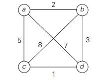
(We solved this problem by exhaustive search in Section 3.4.)

            As a research project, write a report on how state-space trees are used for programming such games as chess, checkers, and tic-tac-toe. The two principal algorithms you should read about are the minimax algorithm and alpha-beta pruning.