Approximation Algorithms for the Traveling Salesman Problem

Approximation Algorithms for the Traveling Salesman Problem

We solved the traveling salesman problem by exhaustive search in Section 3.4, mentioned its decision version as one of the most well-known NP-complete problems in Section 11.3, and saw how its instances can be solved by a branch-and-bound algorithm in Section 12.2. Here, we consider several approximation algorithms, a small sample of dozens of such algorithms suggested over the years for this famous problem. 

But first let us answer the question of whether we should hope to find a polynomial-time approximation algorithm with a finite performance ratio on all instances of the traveling salesman problem. As the following theorem [Sah76] shows, the answer turns out to be no, unless P = N P .

THEOREM 1 If P  != NP, there exists no c-approximation algorithm for the traveling salesman problem, i.e., there exists no polynomial-time approximation algorithm for this problem so that for all instances

PROOF By way of contradiction, suppose that such an approximation algorithm A and a constant c exist. (Without loss of generality, we can assume that c is a positive integer.) We will show that this algorithm could then be used for solving the Hamiltonian circuit problem in polynomial time. We will take advantage of a variation of the transformation used in Section 11.3 to reduce the Hamiltonian circuit problem to the traveling salesman problem. Let G be an arbitrary graph with n vertices. We map G to a complete weighted graph G by assigning weight 1 to each edge in G and adding an edge of weight cn + 1 between each pair of vertices not adjacent in G. If G has a Hamiltonian circuit, its length in G is n; hence, it is the exact solution s^∗ to the traveling salesman problem for G . Note that if s_a is an approximate solution obtained for G by algorithm A, then f (s_a) ≤ cn by the assumption. If G does not have a Hamiltonian circuit in G, the shortest tour in G will contain at least one edge of weight cn + 1, and hence f (s_a) ≥ f (s^∗) > cn. Taking into account the two derived inequalities, we could solve the Hamiltonian circuit problem for graph G in polynomial time by mapping G to G , applying algorithm A to get tour s_a in G , and comparing its length with cn. Since the Hamiltonian circuit problem is NP-complete, we have a contradiction unless P =

NP.

Greedy Algorithms for the TSP The simplest approximation algorithms for the traveling salesman problem are based on the greedy technique. We will discuss here two such algorithms.

Nearest-neighbor algorithm

The following well-known greedy algorithm is based on the nearest-neighbor heuristic: always go next to the nearest unvisited city.

Step 1 Choose an arbitrary city as the start.

Step 2 Repeat the following operation until all the cities have been visited: go to the unvisited city nearest the one visited last (ties can be broken arbitrarily).

Step 3 Return to the starting city.

EXAMPLE 1 For the instance represented by the graph in Figure 12.10, with a as the starting vertex, the nearest-neighbor algorithm yields the tour (Hamiltonian circuit) s_a: a − b − c − d − a of length 10.

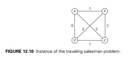
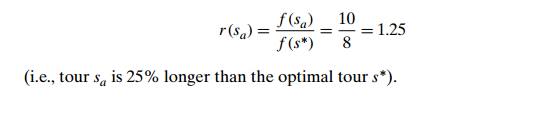
The optimal solution, as can be easily checked by exhaustive search, is the tour s^∗: a − b − d − c − a of length 8. Thus, the accuracy ratio of this approximation is

Unfortunately, except for its simplicity, not many good things can be said about the nearest-neighbor algorithm. In particular, nothing can be said in general about the accuracy of solutions obtained by this algorithm because it can force us to traverse a very long edge on the last leg of the tour. Indeed, if we change the weight of edge (a, d) from 6 to an arbitrary large number w ≥ 6 in Example 1, the algorithm will still yield the tour a − b − c − d − a of length 4 + w, and the optimal solution will still be a − b − d − c − a of length 8. Hence,

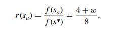
which can be made as large as we wish by choosing an appropriately large value of w. Hence, R_A = ∞ for this algorithm (as it should be according to Theorem 1).

Multifragment-heuristic algorithm

Another natural greedy algorithm for the traveling salesman problem considers it as the problem of finding a minimum-weight collection of edges in a given complete weighted graph so that all the vertices have degree 2. (With this emphasis on edges rather than vertices, what other greedy algorithm does it remind you of?) An application of the greedy technique to this problem leads to the following algorithm [Ben90].

Step 1 Sort the edges in increasing order of their weights. (Ties can be broken arbitrarily.) Initialize the set of tour edges to be constructed to the empty set.

Step 2 Repeat this step n times, where n is the number of cities in the instance being solved: add the next edge on the sorted edge list to the set of tour edges, provided this addition does not create a vertex of degree 3 or a cycle of length less than n; otherwise, skip the edge.

Step 3 Return the set of tour edges.

As an example, applying the algorithm to the graph in Figure 12.10 yields {(a, b), (c, d), (b, c), (a, d)}. This set of edges forms the same tour as the one pro-duced by the nearest-neighbor algorithm. In general, the multifragment-heuristic algorithm tends to produce significantly better tours than the nearest-neighbor algorithm, as we are going to see from the experimental data quoted at the end of this section. But the performance ratio of the multifragment-heuristic algorithm is also unbounded, of course.

There is, however, a very important subset of instances, called Euclidean, for which we can make a nontrivial assertion about the accuracy of both the nearest-neighbor and multifragment-heuristic algorithms. These are the instances in which intercity distances satisfy the following natural conditions:

triangle inequality d[i, j ] ≤ d[i, k] + d[k, j ] for any triple of cities i, j, and k (the distance between cities i and j cannot exceed the length of a two-leg path from i to some intermediate city k to j )

symmetry d[i, j ] = d[j, i] for any pair of cities i and j (the distance from i to j is the same as the distance from j to i)

A substantial majority of practical applications of the traveling salesman prob-lem are its Euclidean instances. They include, in particular, geometric ones, where cities correspond to points in the plane and distances are computed by the standard Euclidean formula. Although the performance ratios of the nearest-neighbor and multifragment-heuristic algorithms remain unbounded for Euclidean instances, their accuracy ratios satisfy the following inequality for any such instance with n ≥ 2 cities:

where f (s_a) and f (s^∗) are the lengths of the heuristic tour and shortest tour, respectively (see [Ros77] and [Ong84]).

Minimum-Spanning-Tree–Based Algorithms There are approximation algori-thms for the traveling salesman problem that exploit a connection between Hamil-tonian circuits and spanning trees of the same graph. Since removing an edge from a Hamiltonian circuit yields a spanning tree, we can expect that the structure of a minimum spanning tree provides a good basis for constructing a shortest tour approximation. Here is an algorithm that implements this idea in a rather straight-forward fashion.

Twice-around-the-tree algorithm

Step 1 Construct a minimum spanning tree of the graph corresponding to a given instance of the traveling salesman problem.

Step 2 Starting at an arbitrary vertex, perform a walk around the minimum spanning tree recording all the vertices passed by. (This can be done by a DFS traversal.)

Step 3 Scan the vertex list obtained in Step 2 and eliminate from it all repeated occurrences of the same vertex except the starting one at the end of the list. (This step is equivalent to making shortcuts in the walk.) The vertices remaining on the list will form a Hamiltonian circuit, which is the output of the algorithm.

EXAMPLE 2 Let us apply this algorithm to the graph in Figure 12.11a. The minimum spanning tree of this graph is made up of edges (a, b), (b, c), (b, d), and (d, e) (Figure 12.11b). A twice-around-the-tree walk that starts and ends at a is

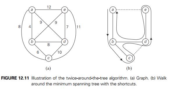
a, b, c, b, d, e, d, b, a.

Eliminating the second b (a shortcut from c to d), the second d, and the third b (a shortcut from e to a) yields the Hamiltonian circuit

a,  b, c, d, e, a

of length 39.

The tour obtained in Example 2 is not optimal. Although that instance is small enough to find an optimal solution by either exhaustive search or branch-and-bound, we refrained from doing so to reiterate a general point. As a rule, we do not know what the length of an optimal tour actually is, and therefore we cannot compute the accuracy ratio f (s_a)/f (s^∗). For the twice-around-the-tree algorithm, we can at least estimate it above, provided the graph is Euclidean.

THEOREM 2 The twice-around-the-tree algorithm is a 2-approximation algo-rithm for the traveling salesman problem with Euclidean distances.

PROOF Obviously, the twice-around-the-tree algorithm is polynomial time if we use a reasonable algorithm such as Prim’s or Kruskal’s in Step 1. We need to show that for any Euclidean instance of the traveling salesman problem, the length of a tour s_a obtained by the twice-around-the-tree algorithm is at most twice the length of the optimal tour s^∗, i.e.,

f (s_a) ≤ 2f (s^∗).

Since removing any edge from s^∗ yields a spanning tree T of weight w(T ), which must be greater than or equal to the weight of the graph’s minimum spanning tree w(T ^∗), we get the inequality

f (s^∗) > w(T ) ≥ w(T ^∗).

This inequality implies that

2f (s^∗) > 2w(T ^∗) = the length of the walk obtained in Step 2 of the algorithm.

The possible shortcuts outlined in Step 3 of the algorithm to obtain s_a cannot increase the total length of the walk in a Euclidean graph, i.e.,

the length of the walk obtained in Step 2 ≥ the length of the tour s_a.

Combining the last two inequalities, we get the inequality

2f (s^∗) > f (s_a),

which is, in fact, a slightly stronger assertion than the one we needed to prove.

Christofides Algorithm There is an approximation algorithm with a better per-formance ratio for the Euclidean traveling salesman problem—the well-known Christofides algorithm [Chr76]. It also uses a minimum spanning tree but does this in a more sophisticated way than the twice-around-the-tree algorithm. Note that a twice-around-the-tree walk generated by the latter algorithm is an Eule-rian circuit in the multigraph obtained by doubling every edge in the graph given. Recall that an Eulerian circuit exists in a connected multigraph if and only if all its vertices have even degrees. The Christofides algorithm obtains such a multi-graph by adding to the graph the edges of a minimum-weight matching of all the odd-degree vertices in its minimum spanning tree. (The number of such vertices is always even and hence this can always be done.) Then the algorithm finds an Eulerian circuit in the multigraph and transforms it into a Hamiltonian circuit by shortcuts, exactly the same way it is done in the last step of the twice-around-the-tree algorithm.

EXAMPLE 3 Let us trace the Christofides algorithm in Figure 12.12 on the same instance (Figure 12.12a) used for tracing the twice-around-the-tree algorithm in Figure 12.11. The graph’s minimum spanning tree is shown in Figure 12.12b. It has four odd-degree vertices: a, b, c, and e. The minimum-weight matching of these four vertices consists of edges (a, b) and (c, e). (For this tiny instance, it can be found easily by comparing the total weights of just three alternatives: (a, b) and (c, e), (a, c) and (b, e), (a, e) and (b, c).) The traversal of the multigraph, starting at vertex a, produces the Eulerian circuit a − b − c − e − d − b − a, which, after one shortcut, yields the tour a − b − c − e − d − a of length 37.

The performance ratio of the Christofides algorithm on Euclidean instances is 1.5 (see, e.g., [Pap82]). It tends to produce significantly better approximations to optimal tours than the twice-around-the-tree algorithm does in empirical tests. (We quote some results of such tests at the end of this subsection.) The quality of a tour obtained by this heuristic can be further improved by optimizing shortcuts made on the last step of the algorithm as follows: examine the multiply-visited cities in some arbitrary order and for each make the best possible shortcut. This 

enhancement would have not improved the tour a − b − c − e − d − a obtained in Example 3 from a − b − c − e − d − b − a because shortcutting the second occur-rence of b happens to be better than shortcutting its first occurrence. In general, however, this enhancement tends to decrease the gap between the heuristic and optimal tour lengths from about 15% to about 10%, at least for randomly gener-ated Euclidean instances [Joh07a].

Local Search Heuristics For Euclidean instances, surprisingly good approxima-tions to optimal tours can be obtained by iterative-improvement algorithms, which are also called local search heuristics. The best-known of these are the 2-opt, 3-opt, and Lin-Kernighan algorithms. These algorithms start with some initial tour, e.g., constructed randomly or by some simpler approximation algorithm such as the nearest-neighbor. On each iteration, the algorithm explores a neighborhood around the current tour by replacing a few edges in the current tour by other edges. If the changes produce a shorter tour, the algorithm makes it the current

tour and continues by exploring its neighborhood in the same manner; otherwise, the current tour is returned as the algorithm’s output and the algorithm stops.

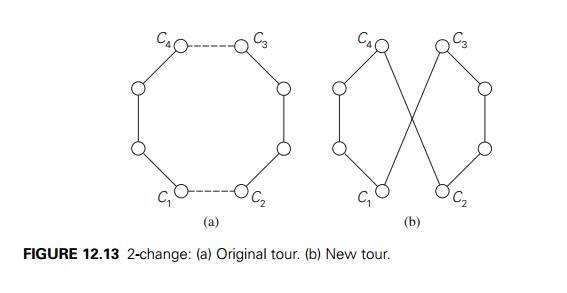
The 2-opt algorithm works by deleting a pair of nonadjacent edges in a tour and reconnecting their endpoints by the different pair of edges to obtain another tour (see Figure 12.13). This operation is called the 2-change. Note that there is only one way to reconnect the endpoints because the alternative produces two disjoint fragments.

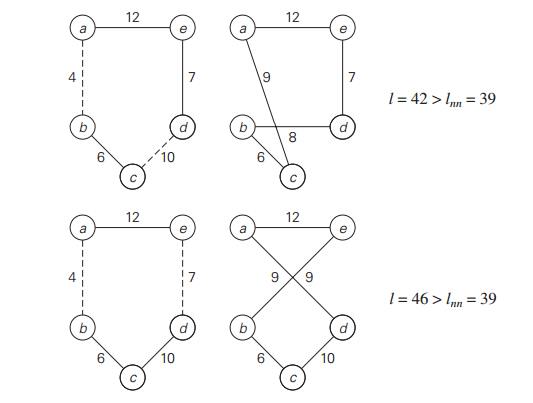
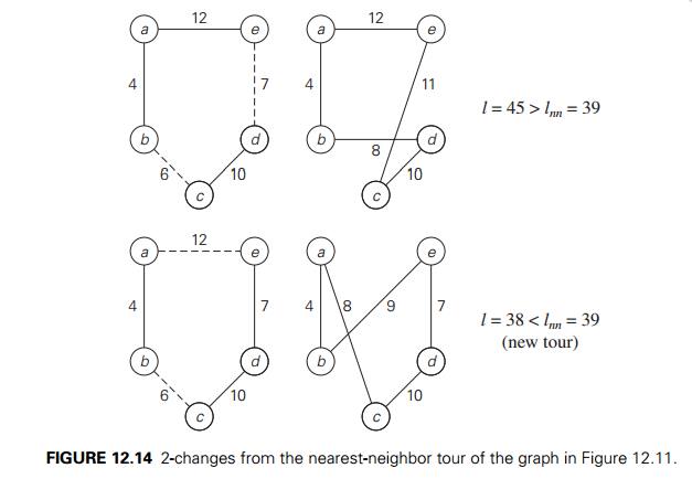
EXAMPLE 4 If we start with the nearest-neighbor tour a − b − c − d − e − a in the graph of Figure 12.11, whose length l_nn is equal to 39, the 2-opt algorithm will move to the next tour as shown in Figure 12.14.

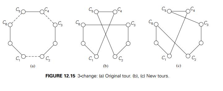
To generalize the notion of the 2-change, one can consider the k-change for any k ≥ 2. This operation replaces up to k edges in a current tour. In addition to 2-changes, only the 3-changes have proved to be of practical interest. The two principal possibilities of 3-changes are shown in Figure 12.15.

There are several other local search algorithms for the traveling salesman problem. The most prominent of them is the Lin-Kernighan algorithm [Lin73], which for two decades after its publication in 1973 was considered the best algo-rithm to obtain high-quality approximations of optimal tours. The Lin-Kernighan algorithm is a variable-opt algorithm: its move can be viewed as a 3-opt move followed by a sequence of 2-opt moves. Because of its complexity, we have to re-frain from discussing this algorithm here. The excellent survey by Johnson and McGeoch [Joh07a] contains an outline of the algorithm and its modern exten-sions as well as methods for its efficient implementation. This survey also contain results from the important empirical studies about performance of many heuris-tics for the traveling salesman problem, including of course, the Lin-Kernighan algorithm. We conclude our discussion by quoting some of these data.

Empirical Results The traveling salesman problem has been the subject of in-tense study for the last 50 years. This interest was driven by a combination of pure theoretical interest and serious practical needs stemming from such newer ap-plications as circuit-board and VLSI-chip fabrication, X-ray crystallography, and genetic engineering. Progress in developing effective heuristics, their efficient im-plementation by using sophisticated data structures, and the ever-increasing power of computers have led to a situation that differs drastically from a pessimistic pic-ture painted by the worst-case theoretical results. This is especially true for the most important applications class of instances of the traveling salesman problem: points in the two-dimensional plane with the standard Euclidean distances be-tween them.

Nowadays, Euclidean instances with up to 1000 cities can be solved exactly in quite a reasonable amount of time—typically, in minutes or faster on a good workstation—by such optimization packages as Concord [App]. In fact, according to the information on the Web site maintained by the authors of that package, the largest instance of the traveling salesman problem solved exactly as of January 2010 was a tour through 85,900 points in a VLSI application. It significantly ex-ceeded the previous record of the shortest tour through all 24,978 cities in Sweden. There should be little doubt that the latest record will also be eventually super-seded and our ability to solve ever larger instances exactly will continue to expand. This remarkable progress does not eliminate the usefulness of approximation al-gorithms for such problems, however. First, some applications lead to instances that are still too large to be solved exactly in a reasonable amount of time. Second, one may well prefer spending seconds to find a tour that is within a few percent of optimum than to spend many hours or even days of computing time to find the shortest tour exactly.

But how can one tell how good or bad the approximate solution is if we do not know the length of an optimal tour? A convenient way to overcome this difficulty is to solve the linear programming problem describing the instance in question by ignoring the integrality constraints. This provides a lower bound—called the Held-Karp bound—on the length of the shortest tour. The Held-Karp bound is typically very close (less than 1%) to the length of an optimal tour, and this bound can be computed in seconds or minutes unless the instance is truly huge. Thus, for a tour

s_a obtained by some heuristic, we estimate the accuracy ratio r(s_a) = f (s_a)/f (s^∗) from above by the ratio f (s_a)/H K(s^∗), where f (s_a) is the length of the heuristic tour s_a and H K(s^∗) is the Held-Karp lower bound on the shortest-tour length.

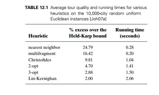
The results (see Table 12.1) from a large empirical study [Joh07a] indicate the average tour quality and running times for the discussed heuristics.³ The instances in the reported sample have 10,000 cities generated randomly and uniformly as integral-coordinate points in the plane, with the Euclidean distances rounded to the nearest integer. The quality of tours generated by the heuristics remain about the same for much larger instances (up to a million cities) as long as they belong to the same type of instances. The running times quoted are for expert implementations run on a Compaq ES40 with 500 Mhz Alpha processors and 2 gigabytes of main memory or its equivalents.

Asymmetric instances of the traveling salesman problem—i.e., those with a nonsymmetic matrix of intercity distances—have proved to be significantly harder to solve, both exactly and approximately, than Euclidean instances. In partic-ular, exact optimal solutions for many 316-city asymmetric instances remained unknown at the time of the state-of-the-art survey by Johnson et al. [Joh07b].