Backtracking

Backtracking

Throughout the book (see in particular Sections 3.4 and 11.3), we have encoun-tered problems that require finding an element with a special property in a domain that grows exponentially fast (or faster) with the size of the problem’s input: a Hamiltonian circuit among all permutations of a graph’s vertices, the most valu-able subset of items for an instance of the knapsack problem, and the like. We addressed in Section 11.3 the reasons for believing that many such problems might not be solvable in polynomial time. Also recall that we discussed in Section 3.4 how such problems can be solved, at least in principle, by exhaustive search. The exhaustive-search technique suggests generating all candidate solutions and then identifying the one (or the ones) with a desired property.

Backtracking is a more intelligent variation of this approach. The principal idea is to construct solutions one component at a time and evaluate such partially constructed candidates as follows. If a partially constructed solution can be de-veloped further without violating the problem’s constraints, it is done by taking the first remaining legitimate option for the next component. If there is no legiti-mate option for the next component, no alternatives for any remaining component need to be considered. In this case, the algorithm backtracks to replace the last component of the partially constructed solution with its next option.

It is convenient to implement this kind of processing by constructing a tree of choices being made, called the state-space tree. Its root represents an initial state before the search for a solution begins. The nodes of the first level in the tree represent the choices made for the first component of a solution, the nodes of the second level represent the choices for the second component, and so on. A node in a state-space tree is said to be promising if it corresponds to a partially constructed solution that may still lead to a complete solution; otherwise,

it is called nonpromising. Leaves represent either nonpromising dead ends or complete solutions found by the algorithm. In the majority of cases, a state-space tree for a backtracking algorithm is constructed in the manner of depth-first search. If the current node is promising, its child is generated by adding the first remaining legitimate option for the next component of a solution, and the processing moves to this child. If the current node turns out to be nonpromising, the algorithm backtracks to the node’s parent to consider the next possible option for its last component; if there is no such option, it backtracks one more level up the tree, and so on. Finally, if the algorithm reaches a complete solution to the problem, it either stops (if just one solution is required) or continues searching for other possible solutions.

n-Queens Problem

As our first example, we use a perennial favorite of textbook writers: the n-queens problem. The problem is to place n queens on an n × n chessboard so that no two queens attack each other by being in the same row or in the same column or on the same diagonal. For n = 1, the problem has a trivial solution, and it is easy to see that there is no solution for n = 2 and n = 3. So let us consider the four-queens problem and solve it by the backtracking technique. 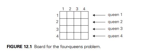Since each of the four queens has to be placed in its own row, all we need to do is to assign a column for each queen on the board presented in Figure 12.1.

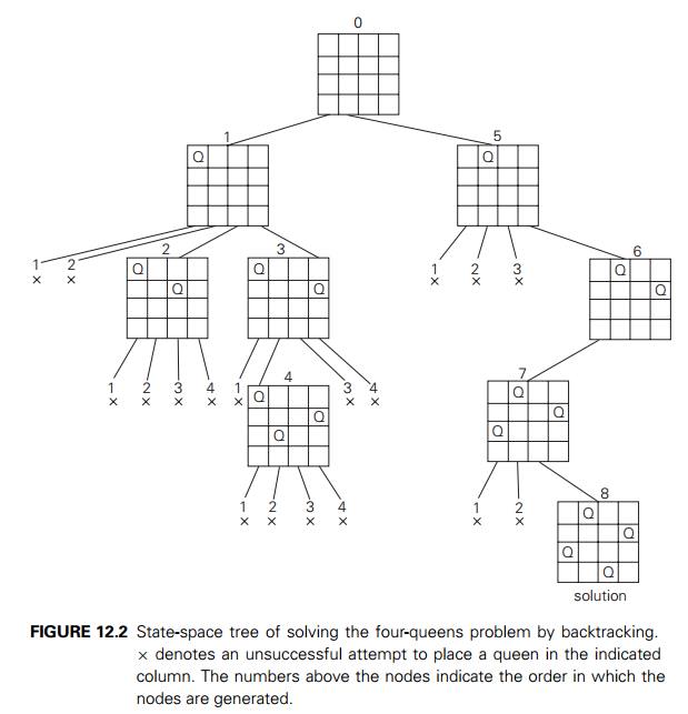
We start with the empty board and then place queen 1 in the first possible position of its row, which is in column 1 of row 1. Then we place queen 2, after trying unsuccessfully columns 1 and 2, in the first acceptable position for it, which is square (2, 3), the square in row 2 and column 3. This proves to be a dead end because there is no acceptable position for queen 3. So, the algorithm backtracks and puts queen 2 in the next possible position at (2, 4). Then queen 3 is placed at (3, 2), which proves to be another dead end. The algorithm then backtracks all the way to queen 1 and moves it to (1, 2). Queen 2 then goes to (2, 4), queen 3 to (3, 1), and queen 4 to (4, 3), which is a solution to the problem. The state-space tree of this search is shown in Figure 12.2.

If other solutions need to be found (how many of them are there for the four-queens problem?), the algorithm can simply resume its operations at the leaf at which it stopped. Alternatively, we can use the board’s symmetry for this purpose.

Finally, it should be pointed out that a single solution to the n-queens problem for any n ≥ 4 can be found in linear time. In fact, over the last 150 years mathe-maticians have discovered several alternative formulas for nonattacking positions of n queens [Bel09]. Such positions can also be found by applying some general algorithm design strategies (Problem 4 in this section’s exercises).

Hamiltonian Circuit Problem

As our next example, let us consider the problem of finding a Hamiltonian circuit in the graph in Figure 12.3a.

Without loss of generality, we can assume that if a Hamiltonian circuit exists, it starts at vertex a. Accordingly, we make vertex a the root of the state-space

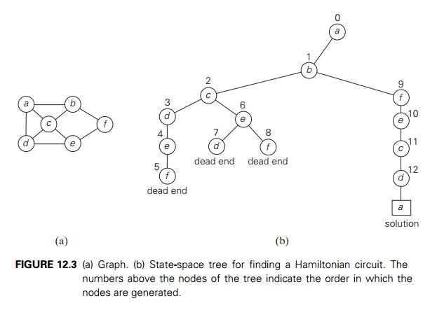
tree (Figure 12.3b). The first component of our future solution, if it exists, is a first intermediate vertex of a Hamiltonian circuit to be constructed. Using the alphabet order to break the three-way tie among the vertices adjacent to a, we select vertex b. From b, the algorithm proceeds to c, then to d, then to e, and finally to f, which proves to be a dead end. So the algorithm backtracks from f to e, then to d, and then to c, which provides the first alternative for the algorithm to pursue. Going from c to e eventually proves useless, and the algorithm has to backtrack from e to c and then to b. From there, it goes to the vertices f , e, c, and d, from which it can legitimately return to a, yielding the Hamiltonian circuit a, b, f , e, c, d, a. If we wanted to find another Hamiltonian circuit, we could continue this process by backtracking from the leaf of the solution found.

Subset-Sum Problem

As our last example, we consider the subset-sum problem: find a subset of a given set A = {a₁, . . . , a_n} of n positive integers whose sum is equal to a given positive integer d. For example, for A = {1, 2, 5, 6, 8} and d = 9, there are two solutions: {1, 2, 6} and {1, 8}. Of course, some instances of this problem may have no solutions.

It is convenient to sort the set’s elements in increasing order. So, we will assume that

a₁ < a₂ < ^{. . .} < a_n.

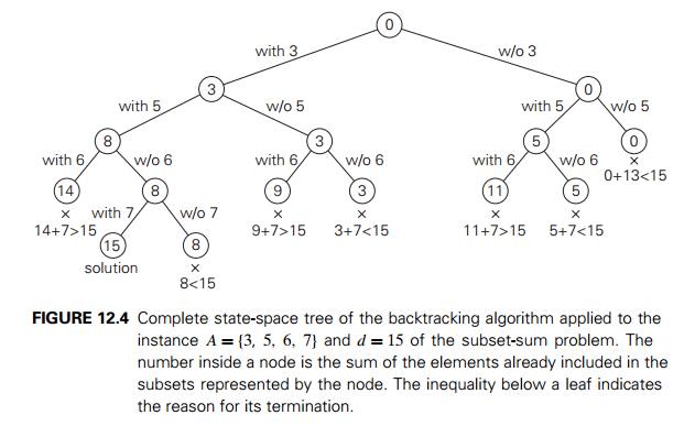
The state-space tree can be constructed as a binary tree like that in Figure 12.4 for the instance A = {3, 5, 6, 7} and d = 15. The root of the tree represents the starting point, with no decisions about the given elements made as yet. Its left and right children represent, respectively, inclusion and exclusion of a₁ in a set being sought. Similarly, going to the left from a node of the first level corresponds to inclusion of a₂ while going to the right corresponds to its exclusion, and so on. Thus, a path from the root to a node on the ith level of the tree indicates which of the first i numbers have been included in the subsets represented by that node.

We record the value of s, the sum of these numbers, in the node. If s is equal to d, we have a solution to the problem. We can either report this result and stop or, if all the solutions need to be found, continue by backtracking to the node’s parent. If s is not equal to d, we can terminate the node as nonpromising if either of the following two inequalities holds:

General Remarks

From a more general perspective, most backtracking algorithms fit the follow-ing description. An output of a backtracking algorithm can be thought of as an n-tuple (x₁, x₂, . . . , x_n) where each coordinate x_i is an element of some finite linearly ordered set S_i. For example, for the n-queens problem, each S_i is the set of integers (column numbers) 1 through n. The tuple may need to satisfy some additional constraints (e.g., the nonattacking requirements in the n-queens prob-lem). Depending on the problem, all solution tuples can be of the same length (the n-queens and the Hamiltonian circuit problem) and of different lengths (the subset-sum problem). A backtracking algorithm generates, explicitly or implic-itly, a state-space tree; its nodes represent partially constructed tuples with the first i coordinates defined by the earlier actions of the algorithm. If such a tuple (x₁, x₂, . . . , x_i) is not a solution, the algorithm finds the next element in S_i+1 that is consistent with the values of (x₁, x₂, . . . , x_i) and the problem’s constraints, and adds it to the tuple as its (i + 1)st coordinate. If such an element does not exist, the algorithm backtracks to consider the next value of x_i, and so on.

To start a backtracking algorithm, the following pseudocode can be called for i = 0 ; X[1..0] represents the empty tuple.

ALGORITHM     Backtrack(X[1..i])

//Gives a template of a generic backtracking algorithm

//Input: X[1..i] specifies first i promising components of a solution //Output: All the tuples representing the problem’s solutions

if X[1..i] is a solution write X[1..i]

else        //see Problem 9 in this section’s exercises

for each element x ∈ S_i+1 consistent with X[1..i] and the constraints do

X[i + 1] ← x

Backtrack(X[1..i + 1])

Our success in solving small instances of three difficult problems earlier in this section should not lead you to the false conclusion that backtracking is a very efficient technique. In the worst case, it may have to generate all possible candidates in an exponentially (or faster) growing state space of the problem at hand. The hope, of course, is that a backtracking algorithm will be able to prune enough branches of its state-space tree before running out of time or memory or both. The success of this strategy is known to vary widely, not only from problem to problem but also from one instance to another of the same problem.

There are several tricks that might help reduce the size of a state-space tree. One is to exploit the symmetry often present in combinatorial problems. For example, the board of the n-queens problem has several symmetries so that some solutions can be obtained from others by reflection or rotation. This implies, in particular, that we need not consider placements of the first queen in the last n/2 columns, because any solution with the first queen in square (1, i), n/2 ≤ i ≤ n, can be obtained by reflection (which?) from a solution with the first queen in square (1, n − i + 1). This observation cuts the size of the tree by about half. Another trick is to preassign values to one or more components of a solution, as we did in the Hamiltonian circuit example. Data presorting in the subset-sum example demonstrates potential benefits of yet another opportunity: rearrange data of an instance given.

It would be highly desirable to be able to estimate the size of the state-space tree of a backtracking algorithm. As a rule, this is too difficult to do analytically, however. Knuth [Knu75] suggested generating a random path from the root to a leaf and using the information about the number of choices available during the path generation for estimating the size of the tree. Specifically, let c₁ be the number of values of the first component x₁ that are consistent with the problem’s constraints. We randomly select one of these values (with equal probability 1/c₁) to move to one of the root’s c₁ children. Repeating this operation for c₂ possible values for x₂ that are consistent with x₁ and the other constraints, we move to one of the c₂ children of that node. We continue this process until a leaf is reached after randomly selecting values for x₁, x₂, . . . , x_n. By assuming that the nodes on level i have c_i children on average, we estimate the number of nodes in the tree as

1 + c₁ + c₁c₂ + ^{. . .} + c₁c₂ ^{. . .} c_n.

Generating several such estimates and computing their average yields a useful estimation of the actual size of the tree, although the standard deviation of this random variable can be large.

In conclusion, three things on behalf of backtracking need to be said. First, it is typically applied to difficult combinatorial problems for which no efficient algo-rithms for finding exact solutions possibly exist. Second, unlike the exhaustive-search approach, which is doomed to be extremely slow for all instances of a problem, backtracking at least holds a hope for solving some instances of nontriv-ial sizes in an acceptable amount of time. This is especially true for optimization problems, for which the idea of backtracking can be further enhanced by evaluat-ing the quality of partially constructed solutions. How this can be done is explained in the next section. Third, even if backtracking does not eliminate any elements of a problem’s state space and ends up generating all its elements, it provides a specific technique for doing so, which can be of value in its own right.

Exercises 12.1

            a. Continue the backtracking search for a solution to the four-queens prob-lem, which was started in this section, to find the second solution to the problem.

            Explain how the board’s symmetry can be used to find the second solution to the four-queens problem.

            a. Which is the last solution to the five-queens problem found by the back-tracking algorithm?

Use the board’s symmetry to find at least four other solutions to the problem.

            a. Implement the backtracking algorithm for the n-queens problem in the lan-guage of your choice. Run your program for a sample of n values to get the numbers of nodes in the algorithm’s state-space trees. Compare these num-bers with the numbers of candidate solutions generated by the exhaustive-search algorithm for this problem (see Problem 9 in Exercises 3.4).

            For each value of n for which you run your program in part (a), estimate the size of the state-space tree by the method described in Section 12.1 and compare the estimate with the actual number of nodes you obtained.

            Design a linear-time algorithm that finds a solution to the n-queens problem for any n ≥ 4.

Apply backtracking to the problem of finding a Hamiltonian circuit in the following graph.

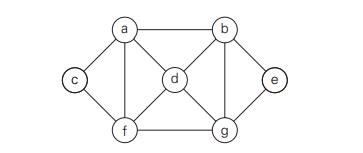
            Apply backtracking to solve the 3-coloring problem for the graph in Fig-ure 12.3a.

            Generate all permutations of {1, 2, 3, 4} by backtracking.

            a. Apply backtracking to solve the following instance of the subset sum problem: A = {1, 3, 4, 5} and d = 11.

            Will the backtracking algorithm work correctly if we use just one of the two inequalities to terminate a node as nonpromising?

            The general template for backtracking algorithms, which is given in the sec-tion, works correctly only if no solution is a prefix to another solution to the problem. Change the template’s pseudocode to work correctly without this restriction.

            Write a program implementing a backtracking algorithm for

            the Hamiltonian circuit problem.

            the m-coloring problem.

Puzzle pegs This puzzle-like game is played on a board with 15 small holes arranged in an equilateral triangle. In an initial position, all but one of the holes are occupied by pegs, as in the example shown below. A legal move is a jump of a peg over its immediate neighbor into an empty square opposite; the jump removes the jumped-over neighbor from the board.

Design and implement a backtracking algorithm for solving the following versions of this puzzle.

            Starting with a given location of the empty hole, find a shortest sequence of moves that eliminates 14 pegs with no limitations on the final position of the remaining peg.

            Starting with a given location of the empty hole, find a shortest sequence of moves that eliminates 14 pegs with the remaining peg at the empty hole of the initial board.