Bewley Lattice Diagram

Bewley Lattice Diagram

This is a convenient diagram devised by Bewley, which shows at a glance the position and direction of motion of every incident, reflected, and transmitted wave on the system at every instant of time. The diagram overcomes the difficulty of otherwise keeping track of the multiplicity of successive reflections at the various junctions.

Consider a transmission line having a resistance r, an inductance l, a conductance g and a capacitance c, all per unit length.

If γ is the propagation constant of the transmission line, and E is the magnitude of the voltage surge at the sending end, then the magnitude and phase of the wave as it reaches any section distance x from the sending end is Ex given by.

where

e - represents the attenuation in the length of line x

e-^j - represents the phase angle change in the length of line x Therefore,

attenuation constant of the line in neper/km phase angle constant of the line in rad/km.

It is also common for an attenuation factor k to be defined corresponding to the length of a particular line. i.e.

k = e for a line of length l.

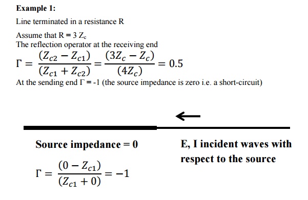
When a voltage surge of magnitude unity reaches a junction between two sections with surge impedances Z₁ and Z₂, then a part is transmitted and a part is reflected back. In traversing the second line, if the attenuation factor is k, then on reaching the termination at the end of the second line its amplitude would be reduced. The lattice diagram may now be constructed as follows. Set the ends of the lines at intervals equal to the time of transit of each line. If a suitable time scale is chosen, then the diagonals on the diagram show the passage of the waves.

  In the Bewley lattice diagram, the following properties exist.

·        All waves travel downhill, because time always increases.

·        The position of any wave at any time can be deduced directly from the diagram.

·        The total potential at any point, at any instant of time is the superposition of all the waves which have arrived at that point up until that instant of time, displaced in position from each other by intervals equal to the difference in their time of arrival.

·        The history of the wave is easily traced. It is possible to find where it came from and just what other waves went into its composition.

·        Attenuation is included, so that the wave arriving at the far end of a line corresponds to the value entering multiplied by the attenuation factor of the line.

This is a diagram which shows at a glance the position and direction of motion of every incident, reflected and transmitted wave on the system at every instant of time. Providing that the system  of lines is not too complex the difficulty of keeping track of the multiplicity of successive reflections is simplified. As a first example, consider the case of an open-circuited line having the following parameters: 

Assume also that RC = GL; this condition (Heaviside condition) results in a distortionless line and the voltage and current waves remain of similar shape in spite of attenuation. In such a line,  it can be shown that if a wave of amplitude A at any point of the line, the amplitude Ax at some  point distant x from the original point is 

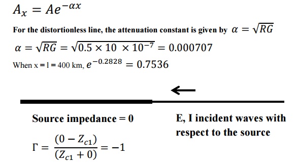
At the receiving end, the line is open-circuited and Ѓ = +1.

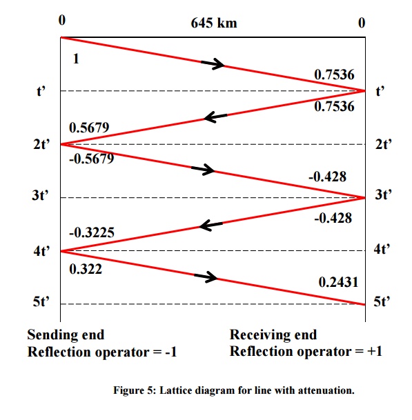
Let us denote the initial value of the voltage at the sending (generating) end by 1 p.u., then, we  will have the following sequence of events as far as the reflected wave is concerned. Let t’ be  the time taken to make one tour of the line, i.e. 400/3×105 zero time, a wave of amplitude 1 starts from G. At time t’, a wave of amplitude 0.7536 reaches  the open end and a reflected wave of amplitude 0.7536 commences the return journey. At time  2t’, this reflected wave is attenuated to 0.5679 and has reached G. Here it is reflected to -0.5679  and after a time 3t’ it reaches the open end attenuated to -0.428. It is then reflected and reaches  G after a time 4t’ with an amplitude of -0.3225. It is then reflected with change of sign thus  starting with an amplitude of 0.3225 and so on. The Bewley lattice diagram is a space-time  diagram with space measured horizontally and time vertically and the lattice of the above  example is shown in Figure 5. The final voltage at the receiving end is the sum to infinity of all  such increments. Thus, in the above example, it is:

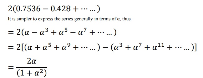
When the given values are substituted in the above expression its value is 0.9613.

Thus, even when open-circuited, such a line gives a far end voltage less than the sending end  voltage, the reason being that the shunt conductance current produces a drop in the series  resistance.