Analysis of data - Economics and Financing of Aquaculture

Analysis of data

Economic analysis of farm performance can be used for a number of purposes. In the allie field of agriculture, the main aims of such studies have been described by Yang (1965) as (i) determination of the relative profitability of various farm enterprises, (ii) assessment of causes or reasons for variation in the unit costs of production, (iii) establishment of efficiency and management standards, (iv) description of the most efficient practices and techniques of farm operation, and (v) determination of the optimum input requirements for each farm enterprise. Taking into account the present state of fish farm economics, Berge (1979) suggested that analysis of data on costs and earnings serve the purpose of (i) helping managers of farms in systematically and realistically studying their own operations, (ii) facilitating comparisons between farms, forming the basis for entrepreneurial decisions on matters such as improvements in the efficiency of the enterprise, and (iii) providing the basis for policy decisions relating to fish farming and facilitating cooperative action with regard to marketing, supply of feed and stocking material, etc. Shang (1981) emphasized that cost and earnings analysis would provide the information necessary to determine the relative profitability of various production techniques or systems, compare the productivity of major inputs, such as land, labour and capital, with that of alternative production activities, and improve the efficiency of the farm operations. He also underlined that the results of economic analy-sis are not only for fish farmers or aquaculturists, ‘but also for economists and policy makers, who make comparisons among different farm groups classified by size, ownership and so on’. Since the normal cost-return analysis is static, he suggested that variations and interactions of factors affecting production and profit should also be considered. ‘Cross-section data collected from a survey can be analysed by regression methods.’ For example, the yield per hectare can be a function of the capital input, man-days employed, amount of feed or fertilizer used, farm size, level of technology, etc. Useful information on how the various factors affect production levels can be obtained from the magnitude of the regression coefficients.

Despite the usefulness of economic evaluation in the development of suitable aquaculture technologies and production programmes, investment appraisals and farm management,

its potential has not yet been utilized to any great extent for reasons already indicated. Recognizing this, some attention is now being paid to this neglected aspect of aquaculture science. Documented data on the operations of individual farms or production systems are now becoming available for certain areas, and these have been used in determining profitability and rates of return on investments and sensitivity studies. Some of the available information will be referred in descriptions of specific farming techniques. A review of available reports would show that, even now, evaluations are frequently based on hypothetical and assumed values which have not been validated by actual case studies or farm surveys.

The methods of economic analyses are described in standard textbooks, but those that have been considered as applicable to aquaculture are summarized here.

Evaluation of farm performance

The basic data required for farm performance analysis, as proposed by Shang (1981), are capital costs, annual operating costs and gross revenue (income). The indicators of performance are as follows:

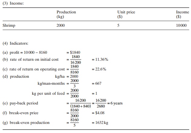
1)       Profit, which is defined as the difference between the gross revenue and the total annual operating cost of production.

2)       Rate of return on investment, which can be derived by dividing the profit by the total investment on fixed assets.

3)       Rate of return on annual operating cost, which is obtained by dividing the profit by the total operating cost.

4)       Value of production per unit of major input. This can be expressed as the weight of production per unit area of water surface or volume of water (kg/ha or kg/m3), weight of production per man-month, weight of production per unit of feed, or unit of capital, etc. These values may partially indicate the operational efficiency.

5)       Cost of input per unit of production; for example cost per kg, man-hour per kg, feed per kg, etc.

6)       Pay-back period, which is the number of years required to recover the investment.

7)       Break-even point, which can be defined as the amount of income where the income (minus variable costs) is sufficient to cover the fixed costs, and there will be no profit and no loss. The break-even price will then be the total operating cost divided by the quantity of production, and the break-even production the total operating cost divided by the unit price of the product.

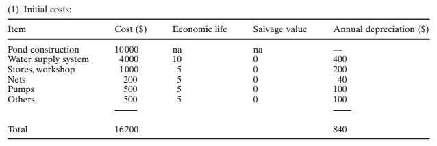
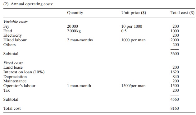
A simplified example of the cost-return analysis of a 1ha shrimp farm partly based on Shang (unpublished) is given below:

Such evaluations to determine the economic performance of a farm or to compare the economic aspects of different farm management systems, as for example extensive versus semi-intensive or intensive, or mono-culture versus polyculture, have been used in many instances.

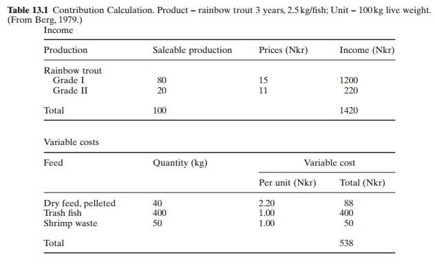
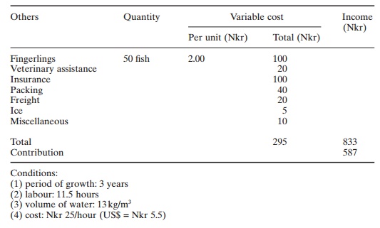
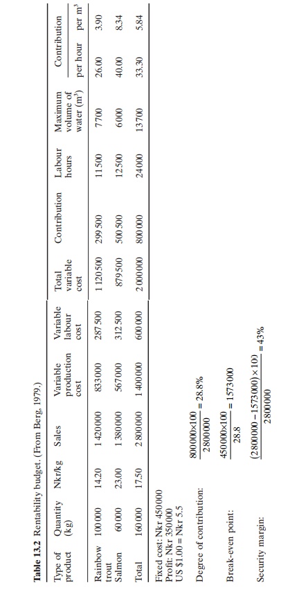
Berg (1979) proposed the use of ‘contribution’ for fish farm accounting, i.e. the operating income minus variable costs, which indicates what remains of the income for fixed costs and net income. This method distinguishes fixed costs from direct variable costs throughout the analysis. Three key values can be calculated by this method:

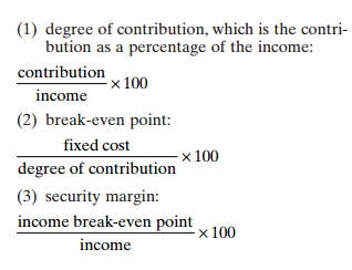
Berg recommended this method of accounting for comparison of different aquaculture enterprises and for working out key indicators for rentability, liquidity, solvency, etc. Examples of calculations of contribution and rentability budget, taken from Berg (1979), are reproduced in Tables 13.1 and 13.2 respectively.

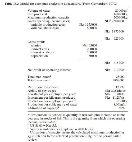
There are also other methods of economic analysis. Gerhardsen (1979) proposed a simple model which can be used for analysing a specific type of production, the total production of an enterprise or the total production of a region. While return on investment is the most common measure of profitability, another useful measure in certain situations is the ability to pay wages. Both measure the same performance, but from different points of view.

The suggested model, based on fish production of a hypothetical aquaculture enterprise in Norway, is reproduced in Table 13.3. Other useful economic indicators which can be calculated from this model are (i) investment per annual man-hours and per kg produced, which indicate the capital intensiveness of the enterprise, (ii) production per annual man-hours, which measures its productivity, and (iii) production per volume or surface unit of water, which indicates the level of intensity of the operation.

Sensitivity analysis

The analysis referred to earlier is static and describes a given situation. It will often be necessary to examine the effect of variations and interactions of factors influencing income and variable costs. In planning and managing an aquaculture enterprise, there will be a continuing need to evaluate the sensitivity of return on investment to changes in major production costs, as well as price of products. Variations in costs may arise from changes in the costs of inputs or the adoption of new technologies. Before introducing new techniques, as realistic an analysis as possible has to be carried out to indicate the capital intensiveness of the enterprise, (ii) production per annual man-hours, which measures its productivity, and (iii) production per volume or surface unit of water, which indicates the level of intensity of the operation.

assess their impact on operating costs. Variations in price can be expected as a result of changes in demand, increased supplies and competition. In the case of export products, changes in foreign market conditions, including currency exchange rates and import regulations, will have a considerable impact on income. It will also be necessary to examine whether the farming of species meant for export can be maintained if the export market ceases to exist and the product has to be sold in the domestic market at lower prices. Fall-back positions in terms of technology, diversification of species and product development and their effects on profitability will have to be worked out.

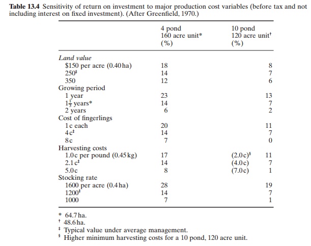
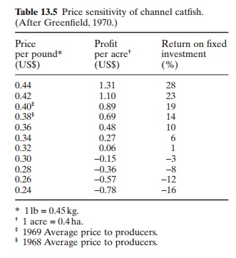
As an example of sensitivity analysis, evaluations of catfish production costs and prices are reproduced in Tables 13.4 and 13.5 from Greenfield (1970).

When there is only a minor change in a production system, which results in a partial change in cost and returns, complete recalculation of economic viability can be avoided by using the partial budgeting method. In this method the benefits are first estimated by the increase in income due to the change, ignoring incomes that will not change. Then the reduction in cost if one proceeds with the venture with the changes is estimated. The next step is

to estimate the added cost due to the change, again ignoring the costs that will not be affected. Then the income foregone due to the change has to be estimated. Finally, the sum of the increased cost should be subtracted from the sum of increased benefits. A positive result would show the profitability of the change anda negative result the loss in profitability due to the change.

Minimum farm size

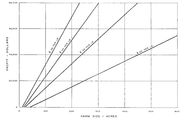
An important decision in a commercial aquaculture venture is the minimum economic size of the farm. Economies of scale are associated with mass production and large-scale enterprises. In many instances, when all inputs are doubled, the output may be more than doubled, showing what is known as increasing return to scale. Economies of scale are generally characterized by the use of higher levels of capital and technology per man-year and a low number of working hours per unit produced. Whether to use the economies of scale or not will depend on the objectives or targets of the project. But in most cases, it will be necessary to determine the minimum size of operation to ensure its economic viability. An investor or a farmer will have to evaluate various farm size combinations to determine the effect of size on production costs and profit. As an example, the study of Mitchell and Usry (1967) on catfish farming in Mississippi (USA) can be cited. Based on the comparison of the prevailing production costs and profits, they came to the conclusion that a new farming operation as small as 30 acres (12.14ha) with a total investment of about $40000 can make a profit in a few years. The summary of results given in Table 13.6 and fig. 13.1 show the decrease in production costs for a farm up to 500 acres in size.

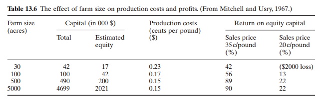
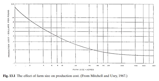
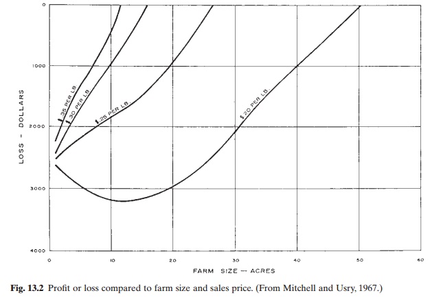
The profit or loss compared to farm size and sale price (fig. 13.2) show that a 500 acre (202.34 ha) farm (requiring $490000 total investment) will have very competitive costs compared to farms of even 5000 acres (2023.4ha). The production costs fall rapidly as the farm size and consequently the investment increase. A $25000 investment was found to produce at a cost of approximately 34 cents a pound and a $100000 investment would bring production costs down to about 17 cents per pound. To get production costs down to 15 cents per pound, an investment of $250000 is required.