Chapter: Transmission Lines and Waveguides : Transmission Line Theory
The Transmission Line , General Solutions & The Infinite Line
THE TRANSMISSION LINE , GENERAL SOLUTIONS & THE INFINITE LINE
A finite line is a line having a finite length on the line. It is a line, which is terminated, in its characteristic impedance (ZR=Z0), so the input impedance of the finite line is equal to the characteristic impedance (Zs=Z0).
An infinite line is a line in which the length of the transmission line is infinite. A finite line, which is terminated in its characteristic impedance, is termed as infinite line. So for an infinite line, the input impedance is equivalent to the characteristic impedance.
The Symmetrical T Network:
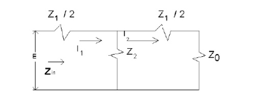
The value of ZO (image impedance) for a symmetrical network can be easily determined. For the symmetrical T network of Fig. 1, terminated in its image impedance ZO, and if Z1 = Z2 = ZT
General solution of the transmission line:
It is used to find the voltage and current at any points on the transmission line. Transmission lines behave very oddly at high frequencies. In traditional (low-frequency) circuit theory, wires connect devices, but have zero resistance. There is no phase delay across wires; and a short-circuited line always yields zero resistance.
For high-frequency transmission lines, things behave quite differently. For instance, short-circuits can actually have an infinite impedance; open-circuits can behave like short-circuited wires. The impedance of some load (ZL=XL+jYL) can be transformed at the terminals of the transmission line to an impedance much different than ZL. The goal of this tutorial is to understand transmission lines and the reasons for their odd effects.
Let's start by examining a diagram. A sinusoidal voltage source with associated impedance ZS is attached to a load ZL (which could be an antenna or some other device – in the circuit diagram we simply view it as an impedance called a load). The load and the source are connected via a transmission line of length L:
Since antennas are often high-frequency devices, transmission line effects are often VERY important. That is, if the length L of the transmission line significantly alters Zin, then the current into the antenna from the source will be very small. Consequently, we will not be delivering power properly to the antenna.
The same problems hold true in the receiving mode: a transmission line can skew impedance of the receiver sufficiently that almost no power is transferred from the antenna. Hence, a thorough understanding of antenna theory requires an understanding of transmission lines. A great antenna can be hooked up to a great receiver, but if it is done with a length of transmission line at high frequencies, the system will not work properly.
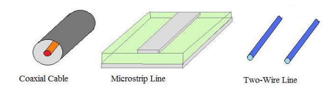
Examples of common transmission lines include the coaxial cable, the microstrip line which commonly feeds patch/microstrip antennas, and the two wire line:
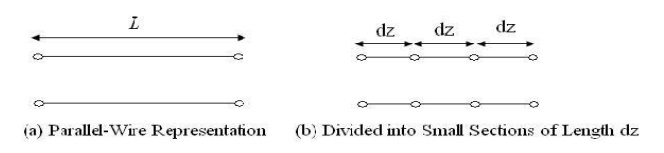
To understand transmission lines, we'll set up an equivalent circuit to model and analyze them. To start, we'll take the basic symbol for a transmission line of length L and divide it into small segments:
Then we'll model each small segment with a small series resistance, series inductance, shunt conductance, and shunt capcitance:
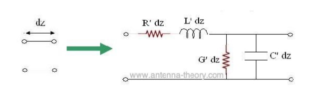
The parameters in the above figure are defined as follows: R' - resistance per unit length for the transmission line (Ohms/meter) L' - inductance per unit length for the tx line (Henries/meter) G' - conductance per unit length for the tx line (Siemans/meter) C' - capacitance per unit length for the tx line (Farads/meter) We will use this model to understand the transmission line. All transmission lines will be represented via the above circuit diagram. For instance, the model for coaxial cables will differ from microstrip transmission lines only by their parameters R', L', G' and C'.
To get an idea of the parameters, R' would represent the d.c. resistance of one meter of the transmission line. The parameter G' represents the isolation between the two conductors of the transmission line. C' represents the capacitance between the two conductors that make up the tx line; L' represents the inductance for one meter of the tx line. These parameters can be derived for each transmission line.
General solutions:
A circuit with distributed parameter requires a method of analysis somewhat different from that employed in circuits of lumped constants. Since a voltage drop occurs across each series increment of a line, the voltage applied to each increment of shunt admittance is a variable and thus the shunted current is a variable along the line.
Hence the line current around the loop is not a constant, as is assumed in lumped constant circuits, but varies from point to point along the line. Differential circuit equations that describes that action will be written for the steady state, from which general circuit equation will be defined as follows.
R= series resistance, ohms per unit length of line( includes both wires)
L= series inductance, henrys per unit length of line
C= capacitance between conductors, faradays per unit length of line
G= shunt leakage conductance between conductors, mhos per unit length Of line
ωL = series reactance, ohms per unit length of line
Z = R+jωL
ωL = series susceptance, mhos per unit length of line
Y = G+jωC
S = distance to the point of observation, measured from the receiving end of the line
I = Current in the line at any point
E= voltage between conductors at any point
l = length of line
The below figure illustrates a line that in the limit may be considered as made up of cascaded infinitesimal T sections, one of which is shown.
This incremental section is of length of ds and carries a current I. The series line impedance being Z ohms and the voltage drop in the length ds is
dE = IZds (1)
dE = IZ (2)
ds
The shunt admittance per unit length of line is Y mhos, so that
The admittance of thr line is Yds mhos. The current dI that follows across the line or from one conductor to the other is
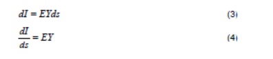
The equation 2 and 4 may be differentiat ed with respwect to s
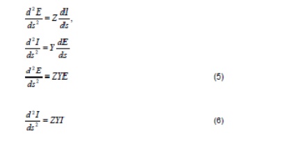
These are the differential equations of the transmission line, fundamental to circuits of distributed constants.
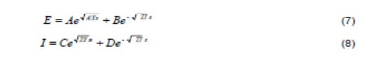
Where A,B,C,D are arbitrary constants of integration.
Since the distance is measured from the receiving end of the line, it is possible to assign conditions such that at
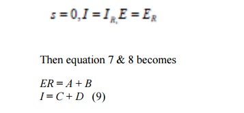
A second set of boundary condition is not available, but the same set may be used over again if a new set of equations are formed by differentiation of equation 7 and 8. Thus
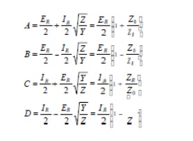
Simultaneous solution of equation 9 ,12 and 13, along with the fact that ER = IRZR and that Z Y has been identified as the Z0 of the line,leads to solution for the constants of the above equations as
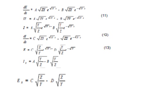
The solution of the differential equations of the transmission line may be written
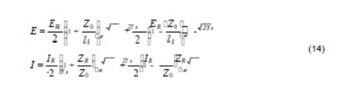
The above equations are very useful form for the voltage and current at any point on a transmission line. After simplifying the above equations we get the final and very useful form of equations for voltage and current at any point on a k=line, and are solutions to the wave equation.
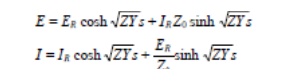
This results indicates two solutions, one for the plus sign and the other for the minus sign before the radical.
Related Topics