Methods of Measuring Secular Trend

Secular trend

It refers to the long term tendency of the data to move in an upward or downward direction. For example, changes in productivity, increase in the rate of capital formation, growth of population, etc ., follow secular trend which has upward direction, while deaths due to improved medical facilities and sanitations show downward trend. All these forces occur in slow process and influence the time series variable in a gradual manner.

Methods of Measuring Trend

Trend is measured using by the following methods:

1. Graphical method

2. Semi averages method

3. Moving averages method

4. Method of least squares

1. Graphical Method

Under this method the values of a time series are plotted on a graph paper by taking time variable on the X-axis and the values variable on the Y-axis. After this, a smooth curve is drawn with free hand through the plotted points. The trend line drawn above can be extended to forecast the values. The following points must be kept in mind in drawing the freehand smooth curve.

(i) The curve should be smooth

(ii) The number of points above the line or curve should be approximately equal to the points below it

(iii) The sum of the squares of the vertical deviation of the points above the smoothed line is equal to the sum of the squares of the vertical deviation of the points below the line.

Merits

·              It is simple method of estimating trend.

·              It requires no mathematical calculations.

·              This method can be used even if trend is not linear.

Demerits

·              It is a subjective method

·              The values of trend obtained by different statisticians would be different and hence not reliable.

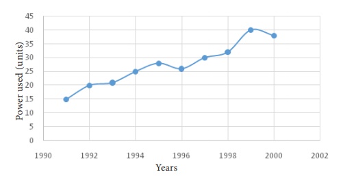
Example 7.1

Annual power consumption per household in a certain locality was reported below.

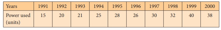
Draw a free hand curve for the above data.

Solution:

2. Semi-Average Method

In this method, the series is divided into two equal parts and the average of each part is plotted at the mid-point of their time duration.

(i) In case the series consists of an even number of years, the series is divisible into two halves. Find the average of the two parts of the series and place these values in the mid-year of each of the respective durations.

(ii) In case the series consists of odd number of years, it is not possible to divide the series into two equal halves. The middle year will be omitted. After dividing the data into two parts, find the arithmetic mean of each part. Thus we get semi-averages.

(iii) The trend values for other years can be computed by successive addition or subtraction for each year ahead or behind any year.

Merits

·              This method is very simple and easy to understand

·              It does not require many calculations.

Demerits

·              This method is used only when the trend is linear.

·              It is used for calculation of averages and they are affected by extreme values.

Example 7.2

Calculate the trend values using semi-averages methods for the income from the forest department. Find the yearly increase.

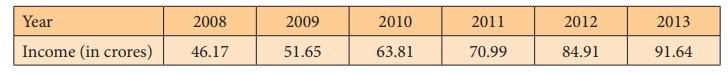
Source: The Principal Chief conservator of forests, Chennai-15.

Solution:

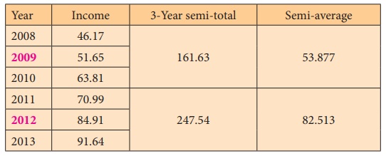
Difference between the central years = 2012 – 2009 = 3 

Difference between the semi-averages = 82.513 – 53.877 = 28.636

Increase in trend value for one year = 28.636 /3 = 9.545

Trend values for the previous and successive years of the central years can be calculated by subtracting and adding respectively, the increase in annual trend value.

Example 7.3

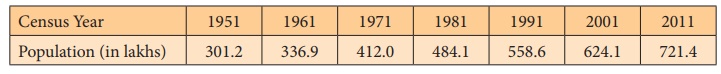
Population of India for 7 successive census years are given below. Find the trend values using semi-averages method.

Solution:

Trend values using semi average method

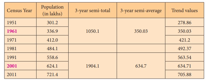
Difference between the years = 2001 – 1961 = 40

Difference between the semi-averages = 634.7 – 350.03 = 284.67

Increase in trend value for 10 year = 284.67 / 4 = 71.17

For example the trend value for the year 1951 = 350.03 – 71.17 = 278.86 The value for the year 2011 = 634.7 + 71.17 = 705.87

The trend values have been calculated by successively subtracting and adding the increase in trend for previous and following years respectively.

Example 7.4

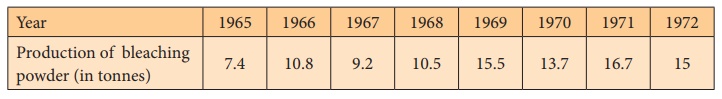
Find the trend values by semi-average method for the following data.

Solution:

Trend values using semi averages method

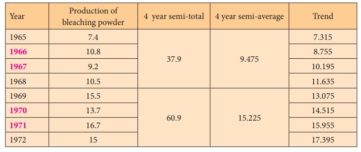
Difference between the years = 1970.5 – 1966.5 = 4

Difference between the semi-averages = 15.225 – 9.475 = 5.75

Increase in trend = 5 .75 / 4 = 1.44

Half yearly increase in trend = 1.44 / 2 = 0.72

The trend value for 1967 = 9.475 + 0.72 = 10.195

The trend value for 1968 = 9.475 + 3 * 0.72 = 11.635

Similarly the trend values for the other years can be calculated.

3. Moving Averages Method

Moving averages is a series of arithmetic means of variate values of a sequence. This is another way of drawing a smooth curve for a time series data.

Moving averages is more frequently used for eliminating the seasonal variations. Even when applied for estimating trend values, the moving average method helps to establish a trend line by eliminating the cyclical, seasonal and random variations present in the time series. The period of the moving average depends upon the length of the time series data.

The choice of the length of a moving average is an important decision in using this method.

For a moving average, appropriate length plays a significant role in smoothening the variations.

In general, if the number of years for the moving average is more then the curve becomes smooth.

Merits

·              It can be easily applied

·              It is useful in case of series with periodic fluctuations.

·              It does not show different results when used by different persons

·              It can be used to find the figures on either extremes; that is, for the past and future years.

Demerits

·              In non-periodic data this method is less effective.

·              Selection of proper ‘period’ or ‘time interval’ for computing moving average is difficult.

·              Values for the first few years and as well as for the last few years cannot be found.

Moving averages odd number of years (3 years)

To find the trend values by the method of three yearly moving averages, the following steps have to be considered.

·              Add up the values of the first 3 years and place the yearly sum against the median year. [This sum is called moving total]

·              Leave the first year value, add up the values of the next three years and place it against its median year.

·              This process must be continued till all the values of the data are taken for calculation.

·              Each 3-yearly moving total must be divided by 3 to get the 3-year moving averages, which is our required trend values.

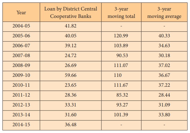
Example 7.5

Calculate the 3-year moving averages for the loans issued by co-operative banks for non-farm sector/small scale industries based on the values given below.

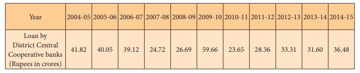
Solution:

The three year moving averages are shown in the last column.

Moving averages - even number of years (4 years)

·              Add up the values of the first 4 years and place the sum against the middle of 2^nd and 3^rd year. (This sum is called 4 year moving total)

·              Leave the first year value and add next 4 values from the 2nd year onward and write the sum against its middle position.

·              This process must be continued till the value of the last item is taken into account.

·              Add the first two 4-years moving total and write the sum against 3rd year.

·              Leave the first 4-year moving total and add the next two 4-year moving total and place it against 4th year.

·              This process must be continued till all the 4-yearly moving totals are summed up and centered.

·              Divide the 4-years moving total by 8 to get the moving averages which are our required trend values.

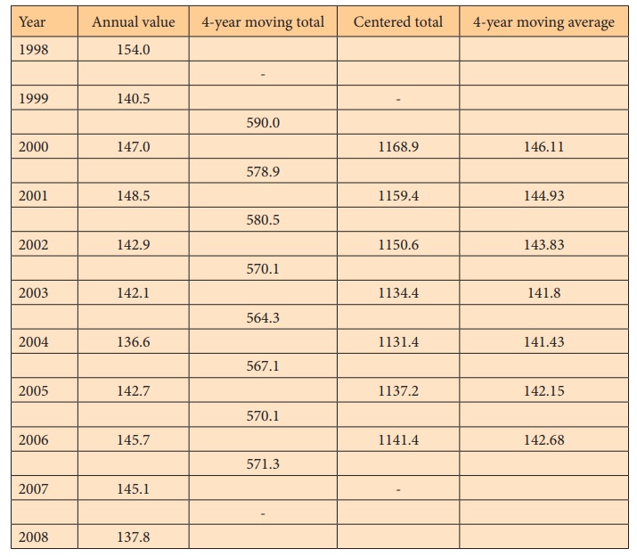
Example 7.6

Compute the trends by the method of moving averages, assuming that 4-year cycle is present in the following series.

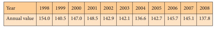
Solution:

The four year moving averages are shown in the last column.

4. Method of least squares

Among the four components of the time series, secular trend represents the long term direction of the series. One way of finding the trend values with the help of mathematical technique is the method of least squares. This method is most widely used in practice and in this method the sum of squares of deviations of the actual and computed values is least and hence the line obtained by this method is known as the line of best fit.

It helps for forecasting the future values. It plays an important role in finding the trend values of economic and business time series data.

Computation of Trend using Method of Least squares

Method of least squares is a device for finding the equation which best fits a given set of observations.

Suppose we are given n pairs of observations and it is required to fit a straight line to these data. The general equation of the straight line is:

y = a + bx

where a and b are constants. Any value of a and b would give a straight line, and once these values are obtained an estimate of y can be obtained by substituting the observed values of y. In order that the equation y = a + b x gives a good representation of the linear relationship between x and y, it is desirable that the estimated values of y_i, say y^{^} _i on the whole close enough to the observed values y_i, i = 1, 2, …, n. According to the principle of least squares, the best fitting equation is obtained by minimizing the sum of squares of differences

is minimum. This leads us to two normal equations.

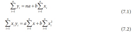
Solving these two equations we get the vales for a and b and the fit of the trend equation (line of best):

y = a + bx (7.3)                  (7.3)

Substituting the observed values x_i in (7.3) we get the trend values y_i, i = 1, 2, …, n.

Note: The time unit is usually of uniform duration and occurs in consecutive numbers. Thus, when the middle period is taken as the point of origin, it reduces the sum of the time variable x to zero  and hence we get

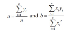
 by simplifying (7.1) and (7.2)

The number of time units may be even or odd, depending upon this, we follow the method of calculating trend values using least square method.

Merits

·              The method of least squares completely eliminates personal bias.

·              Trend values for all the given time periods can be obtained

·              This method enables us to forecast future values.

Demerits

·              The calculations for this method are difficult compared to the other methods.

·              Addition of new observations requires recalculations.

·              It ignores cyclical, seasonal and irregular fluctuations.

·              The trend can be estimated only for immediate future and not for distant future.

Steps for calculating trend values when n is odd:

(i) Subtract the first year from all the years (x)

(ii) Take the middle value (A)

(ii) Find u_i = x_i – A

(iv) Find u_i² and u_iy_i

Then use the normal equations:

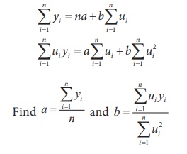
Then the estimated equation of straight line is:

y = a + b u = a + b (x – A)

Example 7.7

Fit a straight line trend by the method of least squares for the following consumer price index numbers of the industrial workers.

Solution:

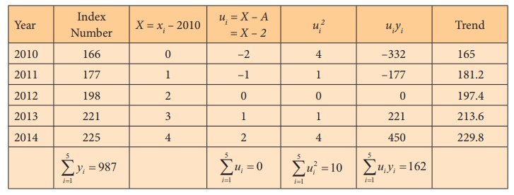
The equation of the straight line is y = a + bx

= a + bu where u = X – 2

The normal equations give:

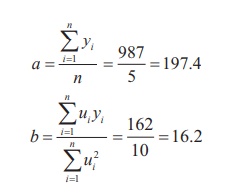
y = 197.4 + 16.2 (X – 2)

= 197.4 + 16.2 X – 32.4

= 16.2 X + 165

That is, y = 165 + 16.2X

To get the required trend values, put X = 0, 1, 2, 3, 4 in the estimated equation.

X = 0, y = 165 + 0 = 165

X = 1, y = 165 + 16.2 = 181.2

X = 2, y = 165 + 32.4 = 197.4

X = 3, y = 165 + 48.6 = 213.6

X = 4, y = 165 + 64.8 = 229.8

Hence, the trend values for 2010, 2011, 2012, 2013 and 2014 are 165, 181.2, 197.4, 213.6 and 229.8 respectively.

Steps for calculating trend values when n is even:

i). Subtract the first year from all the years (x)

ii). Find u_i = 2X – (n – 1)

iii). Find u_i² and u_i y_i

Then follow the same procedure used in previous method for odd years

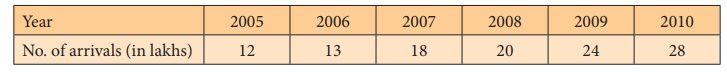
Example 7.8

Tourist arrivals (Foreigners) in Tamil Nadu for 6 consecutive years are given in the following table. Calculate the trend values by using the method of least squares.

Solution:

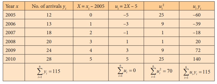
The equation of the straight line is y = a + bx

= a + bu where u = 2X – 5

Using the normal equation we have,

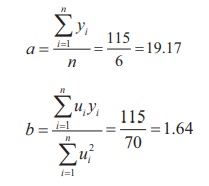
y = a + bu

= 19.17 + 1.64 (2X – 5)

= 19.17 + 3.28X – 8.2

= 3.28X + 10.97

That is, y = 10.97 + 3.28X

To get the required trend values, put X = 0, 1, 2, 3, 4, 5 in the estimated equation. Thus,

X = 0, y = 10.97 + 0 = 10.97

X = 1, y = 10.97 + 3.28 = 14.25

X = 2, y = 10.97 + 6.56 = 17.53

X = 3, y = 10.97 + 9.84 = 20.81

X = 4, y = 10.97 + 13.12 = 24.09

X = 5, y = 10.97 + 16.4 = 27.37

Hence, the trend values for 2005, 2006, 2007, 2008, 2009 and 2010 are 10.97, 14.25, 17.53, 20.81, 24.09 and 27.37 respectively.