Gaussian Elimination

Gaussian Elimination

You are certainly familiar with systems of two linear equations in two unknowns:

a₁₁x + a₁₂y = b₁

a₂₁x + a₂₂y = b₂.

Recall that unless the coefficients of one equation are proportional to the coef-ficients of the other, the system has a unique solution. The standard method for finding this solution is to use either equation to express one of the variables as a function of the other and then substitute the result into the other equation, yield-ing a linear equation whose solution is then used to find the value of the second variable.

In many applications, we need to solve a system of n equations in n unknowns:

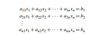
where n is a large number. Theoretically, we can solve such a system by general-izing the substitution method for solving systems of two linear equations (what general design technique would such a method be based upon?); however, the resulting algorithm would be extremely cumbersome.

Fortunately, there is a much more elegant algorithm for solving systems of linear equations called Gaussian elimination.² The idea of Gaussian elimination is to transform a system of n linear equations in n unknowns to an equivalent system (i.e., a system with the same solution as the original one) with an upper-triangular coefficient matrix, a matrix with all zeros below its main diagonal:

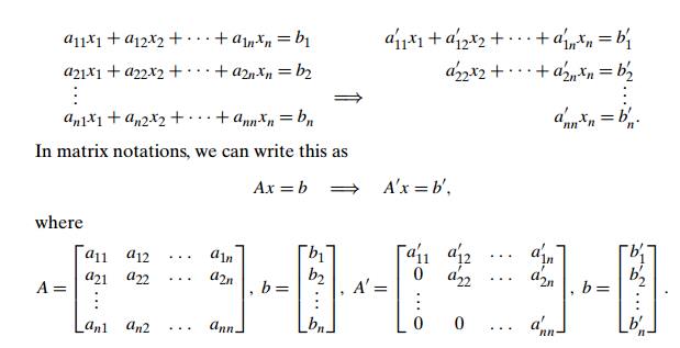
(We added primes to the matrix elements and right-hand sides of the new system to stress the point that their values differ from their counterparts in the original system.)

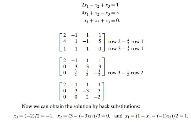
Why is the system with the upper-triangular coefficient matrix better than a system with an arbitrary coefficient matrix? Because we can easily solve the system with an upper-triangular coefficient matrix by back substitutions as follows. First, we can immediately find the value of x_n from the last equation; then we can substitute this value into the next to last equation to get x_n−1, and so on, until we substitute the known values of the last n − 1 variables into the first equation, from which we find the value of x₁.

So how can we get from a system with an arbitrary coefficient matrix A to an equivalent system with an upper-triangular coefficient matrix A ? We can do that through a series of the so-called elementary operations:

exchanging two equations of the system replacing an equation with its nonzero multiple replacing an equation with a sum or difference of this equation and some multiple of another equation

Since no elementary operation can change a solution to a system, any system that is obtained through a series of such operations will have the same solution as the original one.

Let us see how we can get to a system with an upper-triangular matrix. First, we use a₁₁ as a pivot to make all x₁ coefficients zeros in the equations below the first one. Specifically, we replace the second equation with the difference between it and the first equation multiplied by a₂₁/a₁₁ to get an equation with a zero coefficient for x₁. Doing the same for the third, fourth, and finally nth equation—with the multiples a₃₁/a₁₁, a₄₁/a₁₁, . . . , a_n1/a₁₁ of the first equation, respectively—makes all the coefficients of x₁ below the first equation zero. Then we get rid of all the coefficients of x₂ by subtracting an appropriate multiple of the second equation from each of the equations below the second one. Repeating this elimination for each of the first n − 1 variables ultimately yields a system with an upper-triangular coefficient matrix.

Before we look at an example of Gaussian elimination, let us note that we can operate with just a system’s coefficient matrix augmented, as its (n + 1)st column, with the equations’ right-hand side values. In other words, we need to write explicitly neither the variable names nor the plus and equality signs.

EXAMPLE 1       Solve the system by Gaussian elimination.

Here is pseudocode of the first stage, called forward elimination, of the algorithm.

ALGORITHM                 ForwardElimination(A[1..n, 1..n], b[1..n])

//Applies Gaussian elimination to matrix A of a system’s coefficients, //augmented with vector b of the system’s right-hand side values //Input: Matrix A[1..n, 1..n] and column-vector b[1..n]

//Output: An equivalent upper-triangular matrix in place of A with the //corresponding right-hand side values in the (n + 1)st column

for i ← 1 to n do A[i, n + 1] ← b[i] //augments the matrix for i ← 1 to n − 1 do

for j ← i + 1 to n do

for k ← i to n + 1 do

A[j, k] ← A[j, k] − A[i, k] ∗ A[j, i] / A[i, i]

There are two important observations to make about this pseudocode. First, it is not always correct: if A[i, i] = 0, we cannot divide by it and hence cannot use the ith row as a pivot for the ith iteration of the algorithm. In such a case, we should take advantage of the first elementary operation and exchange the ith row with some row below it that has a nonzero coefficient in the ith column. (If the system has a unique solution, which is the normal case for systems under consideration, such a row must exist.)

Since we have to be prepared for the possibility of row exchanges anyway, we can take care of another potential difficulty: the possibility that A[i, i] is so small and consequently the scaling factor A[j, i]/A[i, i] so large that the new value of A[j, k] might become distorted by a round-off error caused by a subtraction of two numbers of greatly different magnitudes.³ To avoid this problem, we can always look for a row with the largest absolute value of the coefficient in the ith column, exchange it with the ith row, and then use the new A[i, i] as the ith iteration’s pivot. This modification, called partial pivoting, guarantees that the magnitude of the scaling factor will never exceed 1.

The second observation is the fact that the innermost loop is written with a glaring inefficiency. Can you find it before checking the following pseudocode, which both incorporates partial pivoting and eliminates this inefficiency?

ALGORITHM     BetterForwardElimination(A[1..n, 1..n], b[1..n])

//Implements Gaussian elimination with partial pivoting //Input: Matrix A[1..n, 1..n] and column-vector b[1..n]

//Output: An equivalent upper-triangular matrix in place of A and the //corresponding right-hand side values in place of the (n + 1)st column for i ← 1 to n do A[i, n + 1] ← b[i] //appends b to A as the last column for i ← 1 to n − 1 do

pivot row ← i

for j ← i + 1 to n do

if |A[j, i]| > |A[pivot row, i]| pivot row ← j for k ← i to n + 1 do

swap(A[i, k], A[pivot row, k]) for j ← i + 1 to n do

t emp ← A[j, i] / A[i, i] for k ← i to n + 1 do

A[j, k] ← A[j, k] − A[i, k] ∗ t emp

Let us find the time efficiency of this algorithm. Its innermost loop consists of a single line,

A[j, k] ← A[j, k] − A[i, k] ∗ t emp,

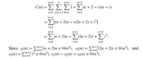
which contains one multiplication and one subtraction. On most computers, multi-plication is unquestionably more expensive than addition/subtraction, and hence it is multiplication that is usually quoted as the algorithm’s basic operation.⁴ The standard summation formulas and rules reviewed in Section 2.3 (see also Appen-dix A) are very helpful in the following derivation:

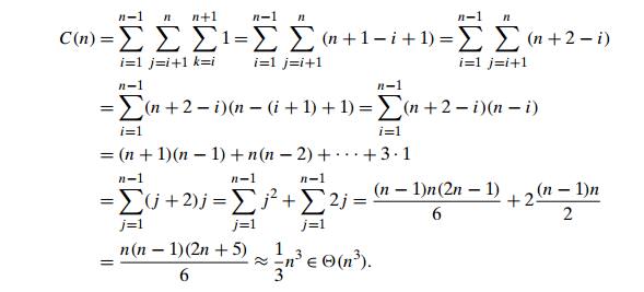
Since the second (back substitution) stage of Gaussian elimination is in  (n²), as you are asked to show in the exercises, the running time is dominated by the cubic elimination stage, making the entire algorithm cubic as well.

Theoretically, Gaussian elimination always either yields an exact solution to a system of linear equations when the system has a unique solution or discovers that no such solution exists. In the latter case, the system will have either no solutions or infinitely many of them. In practice, solving systems of significant size on a computer by this method is not nearly so straightforward as the method would lead us to believe. The principal difficulty lies in preventing an accumulation of round-off errors (see Section 11.4). Consult textbooks on numerical analysis that analyze this and other implementation issues in great detail.

LU Decomposition

Gaussian elimination has an interesting and very useful byproduct called LU de-composition of the coefficient matrix. In fact, modern commercial implementa-tions of Gaussian elimination are based on such a decomposition rather than on the basic algorithm outlined above.

EXAMPLE Let us return to the example in the beginning of this section, where we applied Gaussian elimination to the matrix

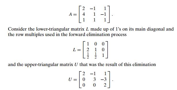
It turns out that the product LU of these matrices is equal to matrix A. (For this particular pair of L and U , you can verify this fact by direct multiplication, but as a general proposition, it needs, of course, a proof, which we omit here.)

Therefore, solving the system Ax = b is equivalent to solving the system LU x = b. The latter system can be solved as follows. Denote y = U x, then Ly = b. Solve the system Ly = b first, which is easy to do because L is a lower-triangular matrix; then solve the system U x = y, with the upper-triangular matrix U , to find x. Thus, for the system at the beginning of this section, we first solve Ly = b:

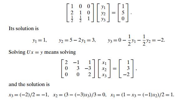
Note that once we have the LU decomposition of matrix A, we can solve systems Ax = b with as many right-hand side vectors b as we want to, one at a time. This is a distinct advantage over the classic Gaussian elimination discussed earlier. Also note that the LU decomposition does not actually require extra memory, because we can store the nonzero part of U in the upper-triangular part of A (including the main diagonal) and store the nontrivial part of L below the main diagonal of A.

Computing a Matrix Inverse

Gaussian elimination is a very useful algorithm that tackles one of the most important problems of applied mathematics: solving systems of linear equations. In fact, Gaussian elimination can also be applied to several other problems of linear algebra, such as computing a matrix inverse. The inverse of an n × n matrix A is an n × n matrix, denoted A⁻¹, such that

AA⁻¹ = I,

where I is the n × n identity matrix (the matrix with all zero elements except the main diagonal elements, which are all ones). Not every square matrix has an inverse, but when it exists, the inverse is unique. If a matrix A does not have an inverse, it is called singular. One can prove that a matrix is singular if and only if one of its rows is a linear combination (a sum of some multiples) of the other rows. A convenient way to check whether a matrix is nonsingular is to apply Gaussian elimination: if it yields an upper-triangular matrix with no zeros on the main diagonal, the matrix is nonsingular; otherwise, it is singular. So being singular is a very special situation, and most square matrices do have their inverses.

Theoretically, inverse matrices are very important because they play the role of reciprocals in matrix algebra, overcoming the absence of the explicit division operation for matrices. For example, in a complete analogy with a linear equation in one unknown ax = b whose solution can be written as x = a⁻¹b (if a is not zero), we can express a solution to a system of n equations in n unknowns Ax = b as x = A⁻¹b (if A is nonsingular) where b is, of course, a vector, not a number.

According to the definition of the inverse matrix for a nonsingular n × n matrix A, to compute it we need to find n² numbers x_ij , 1 ≤ i, j ≤ n, such that

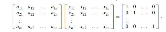
We can find the unknowns by solving n systems of linear equations that have the same coefficient matrix A, the vector of unknowns x^j is the j th column of the inverse, and the right-hand side vector e^j is the j th column of the identity matrix

(1 ≤ j ≤ n):

Ax^j = e^j .

We can solve these systems by applying Gaussian elimination to matrix A aug-mented by the n × n identity matrix. Better yet, we can use forward elimina-tion to find the LU decomposition of A and then solve the systems LU x^j = e^j , j = 1, . . . , n, as explained earlier.

Computing a Determinant

Another problem that can be solved by Gaussian elimination is computing a determinant. The determinant of an n × n matrix A, denoted det A or |A|, is a number whose value can be defined recursively as follows. If n = 1, i.e., if A consists of a single element a₁₁, det A is equal to a₁₁; for n > 1, det A is computed by the recursive formula

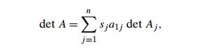
where s_j is +1 if j is odd and −1 if j is even, a_1j is the element in row 1 and column j , and A_j is the (n − 1) × (n − 1) matrix obtained from matrix A by deleting its row 1 and column j .

In particular, for a 2 × 2 matrix, the definition implies a formula that is easy to remember:

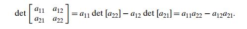
In other words, the determinant of a 2 × 2 matrix is simply equal to the difference between the products of its diagonal elements.

For a 3 × 3 matrix, we get

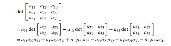
Incidentally, this formula is very handy in a variety of applications. In particular, we used it twice already in Section 5.5 as a part of the quickhull algorithm.

But what if we need to compute a determinant of a large matrix? Although this is a task that is rarely needed in practice, it is worth discussing nevertheless. Using the recursive definition can be of little help because it implies computing the sum of n! terms. Here, Gaussian elimination comes to the rescue again. The central point is the fact that the determinant of an upper-triangular matrix is equal to the product of elements on its main diagonal, and it is easy to see how elementary operations employed by the elimination algorithm influence the determinant’s value. (Basically, it either remains unchanged or changes a sign or is multiplied by the constant used by the elimination algorithm.) As a result, we can compute the determinant of an n × n matrix in cubic time.

Determinants play an important role in the theory of systems of linear equa-tions. Specifically, a system of n linear equations in n unknowns Ax = b has a unique solution if and only if the determinant of its coefficient matrix det A is

not equal to zero. Moreover, this solution can be found by the formulas called

Cramer’s rule,

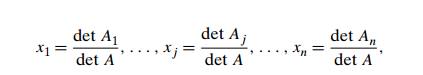
where det A_j is the determinant of the matrix obtained by replacing the j th column of A by the column b. You are asked to investigate in the exercises whether using Cramer’s rule is a good algorithm for solving systems of linear equations.

Exercises 6.2

Q. Solve the following system by Gaussian elimination:

x₁ + x₂ + x₃ = 2 2x₁ + x₂ + x₃ = 3 x₁ − x₂ + 3x₃ = 8.

Q.             a. Solve the system of the previous question by the LU decomposition method.

            From the standpoint of general algorithm design techniques, how would you classify the LU decomposition method?

           Q. Solve the system of Problem 1 by computing the inverse of its coefficient matrix and then multiplying it by the vector on the right-hand side.

Q. Would it be correct to get the efficiency class of the forward elimination stage of Gaussian elimination as follows?

            Write pseudocode for the back-substitution stage of Gaussian elimination and show that its running time is in  (n²).

Assuming that division of two numbers takes three times longer than their multiplication, estimate how much faster BetterForwardElimination is than ForwardElimination. (Of course, you should also assume that a compiler is not going to eliminate the inefficiency in ForwardElimination.)

            Q. a. Give an example of a system of two linear equations in two unknowns that has a unique solution and solve it by Gaussian elimination.

            Give an example of a system of two linear equations in two unknowns that has no solution and apply Gaussian elimination to it.

            Give an example of a system of two linear equations in two unknowns that has infinitely many solutions and apply Gaussian elimination to it.

            Q. The Gauss-Jordan elimination method differs from Gaussian elimination in that the elements above the main diagonal of the coefficient matrix are made zero at the same time and by the same use of a pivot row as the elements below the main diagonal.

            Apply the Gauss-Jordan method to the system of Problem 1 of these exercises.

            What general design strategy is this algorithm based on?

            In general, how many multiplications are made by this method in solving a system of n equations in n unknowns? How does this compare with the number of multiplications made by the Gaussian elimination method in both its elimination and back-substitution stages?

            Q. A system Ax = b of n linear equations in n unknowns has a unique solution if and only if det A  = 0. Is it a good idea to check this condition before applying Gaussian elimination to the system?

           Q. a.  Apply Cramer’s rule to solve the system of Problem 1 of these exercises.

            Estimate how many times longer it will take to solve a system of n linear equations in n unknowns by Cramer’s rule than by Gaussian elimination. Assume that all the determinants in Cramer’s rule formulas are computed independently by Gaussian elimination.

Q.             Lights out This one-person game is played on an n × n board composed of 1 × 1 light panels. Each panel has a switch that can be turned on and off, thereby toggling the on/off state of this and four vertically and horizontally adjacent panels. (Of course, toggling a corner square affects a total of three panels, and toggling a noncorner panel on the board’s border affects a total of four squares.) Given an initial subset of lighted squares, the goal is to turn all the lights off.

            Show that an answer can be found by solving a system of linear equations with 0/1 coefficients and right-hand sides using the modulo 2 arithmetic.

            Use Gaussian elimination to solve the 2 × 2 “all-ones” instance of this problem, where all the panels of the 2 × 2 board are initially lit.

Use Gaussian elimination to solve the 3 × 3 “all-ones” instance of this problem, where all the panels of the 3 × 3 board are initially lit.