B-Trees Algorithms

B-Trees

The idea of using extra space to facilitate faster access to a given data set is partic-ularly important if the data set in question contains a very large number of records that need to be stored on a disk. A principal device in organizing such data sets is an index, which provides some information about the location of records with indicated key values. For data sets of structured records (as opposed to “unstruc-tured” data such as text, images, sound, and video), the most important index organization is the B-tree, introduced by R. Bayer and E. McGreight [Bay72]. It extends the idea of the 2-3 tree (see Section 6.3) by permitting more than a single key in the same node of a search tree.

In the B-tree version we consider here, all data records (or record keys) are stored at the leaves, in increasing order of the keys. The parental nodes are used for indexing. Specifically, each parental node contains n − 1 ordered keys K₁ < ^{. . .} < K_n−1 assumed, for the sake of simplicity, to be distinct. The keys are interposed with n pointers to the node’s children so that all the keys in subtree T₀ are smaller than K₁, all the keys in subtree T₁ are greater than or equal to K₁ and smaller than K₂ with K₁ being equal to the smallest key in T₁, and so on, through the last subtree T_n−1 whose keys are greater than or equal to K_n−1 with K_n−1 being equal to the smallest key in T_n−1 (see Figure 7.7).

In addition, a B-tree of order m ≥ 2 must satisfy the following structural properties:

The root is either a leaf or has between 2 and m children.

Each node, except for the root and the leaves, has between m/2 and m children (and hence between m/2 − 1 and m − 1 keys).

The tree is (perfectly) balanced, i.e., all its leaves are at the same level.

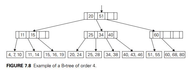
An example of a B-tree of order 4 is given in Figure 7.8.

Searching in a B-tree is very similar to searching in the binary search tree, and even more so in the 2-3 tree. Starting with the root, we follow a chain of pointers to the leaf that may contain the search key. Then we search for the search key among the keys of that leaf. Note that since keys are stored in sorted order, at both parental nodes and leaves, we can use binary search if the number of keys at a node is large enough to make it worthwhile.

It is not the number of key comparisons, however, that we should be con-cerned about in a typical application of this data structure. When used for storing a large data file on a disk, the nodes of a B-tree normally correspond to the disk pages. Since the time needed to access a disk page is typically several orders of magnitude larger than the time needed to compare keys in the fast computer mem-ory, it is the number of disk accesses that becomes the principal indicator of the efficiency of this and similar data structures.

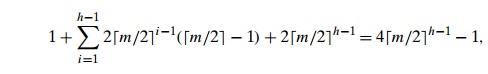
How many nodes of a B-tree do we need to access during a search for a record with a given key value? This number is, obviously, equal to the height of the tree plus 1. To estimate the height, let us find the smallest number of keys a B-tree of order m and positive height h can have. The root of the tree will contain at least one key. Level 1 will have at least two nodes with at least m/2 − 1 keys in each of them, for the total minimum number of keys 2( m/2 − 1). Level 2 will have at least 2 m/2 nodes (the children of the nodes on level 1) with at least m/2 − 1 in each of them, for the total minimum number of keys 2 m/2 ( m/2 − 1). In general, the nodes of level i, 1 ≤ i ≤ h − 1, will contain at least 2 m/2 ⁱ⁻¹( m/2 − 1) keys. Finally, level h, the leaf level, will have at least 2 m/2 ^h−1 nodes with at least one key in each. Thus, for any B-tree of order m with n nodes and height h > 0, we have the following inequality:

After a series of standard simplifications (see Problem 2 in this section’s exercises), this inequality reduces to

which, in turn, yields the following upper bound on the height h of the B-tree of order m with n nodes:

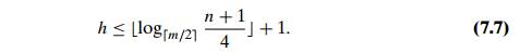
Inequality (7.7) immediately implies that searching in a B-tree is a O(log n) operation. But it is important to ascertain here not just the efficiency class but the actual number of disk accesses implied by this formula. The following table contains the values of the right-hand-side estimates for a file of 100 million records and a few typical values of the tree’s order m:

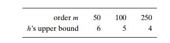
Keep in mind that the table’s entries are upper estimates for the number of disk accesses. In actual applications, this number rarely exceeds 3, with the B-tree’s root and sometimes first-level nodes stored in the fast memory to minimize the number of disk accesses.

The operations of insertion and deletion are less straightforward than search-ing, but both can also be done in O(log n) time. Here we outline an insertion algorithm only; a deletion algorithm can be found in the references (e.g., [Aho83], [Cor09]).

The most straightforward algorithm for inserting a new record into a B-tree is quite similar to the algorithm for insertion into a 2-3 tree outlined in Section 6.3. First, we apply the search procedure to the new record’s key K to find the appropriate leaf for the new record. If there is room for the record in that leaf, we place it there (in an appropriate position so that the keys remain sorted) and we are done. If there is no room for the record, the leaf is split in half by sending the second half of the records to a new node. After that, the smallest key K in the new node and the pointer to it are inserted into the old leaf’s parent (immediately after the key and pointer to the old leaf). This recursive procedure may percolate up to the tree’s root. If the root is already full too, a new root is created with the two halves of the old root’s keys split between two children of the new root. As an example, Figure 7.9 shows the result of inserting 65 into the B-tree in Figure 7.8 under the restriction that the leaves cannot contain more than three items.

You should be aware that there are other algorithms for implementing inser-tions into a B-tree. For example, to avoid the possibility of recursive node splits, we can split full nodes encountered in searching for an appropriate leaf for the new record. Another possibility is to avoid some node splits by moving a key to the node’s sibling. For example, inserting 65 into the B-tree in Figure 7.8 can be done by moving 60, the smallest key of the full leaf, to its sibling with keys 51 and 55, and replacing the key value of their parent by 65, the new smallest value in

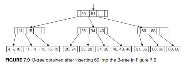
the second child. This modification tends to save some space at the expense of a slightly more complicated algorithm.

A B-tree does not have to be always associated with the indexing of a large file, and it can be considered as one of several search tree varieties. As with other types of search trees—such as binary search trees, AVL trees, and 2-3 trees—a B-tree can be constructed by successive insertions of data records into the initially empty tree. (The empty tree is considered to be a B-tree, too.) When all keys reside in the leaves and the upper levels are organized as a B-tree comprising an index, the entire structure is usually called, in fact, a B⁺-tree.

Exercises 7.4

            Give examples of using an index in real-life applications that do not involve computers.

a.  Prove the equality

which was used in the derivation of upper bound (7.7) for the height of a B-tree.

            Complete the derivation of inequality (7.7).

            Find the minimum order of the B-tree that guarantees that the number of disk accesses in searching in a file of 100 million records does not exceed 3. Assume that the root’s page is stored in main memory.

            Draw the B-tree obtained after inserting 30 and then 31 in the B-tree in Figure 7.8. Assume that a leaf cannot contain more than three items.

            Outline an algorithm for finding the largest key in a B-tree.

a. A top-down 2-3-4 tree is a B-tree of order 4 with the following modifica-tion of the insert operation: Whenever a search for a leaf for a new key

encounters a full node (i.e., a node with three keys), the node is split into two nodes by sending its middle key to the node’s parent, or, if the full node happens to be the root, the new root for the middle key is created. Construct a top-down 2-3-4 tree by inserting the following list of keys in the initially empty tree:

10,                                                  6, 15, 31,      20, 27, 50, 44,         18.

            What is the principal advantage of this insertion procedure compared with the one used for 2-3 trees in Section 6.3? What is its disadvantage?

            a.  Write a program implementing a key insertion algorithm in a B-tree.

            Write a program for visualization of a key insertion algorithm in a B-tree.

SUMMARY

Space and time trade-offs in algorithm design are a well-known issue for both theoreticians and practitioners of computing. As an algorithm design technique, trading space for time is much more prevalent than trading time for space.

Input enhancement is one of the two principal varieties of trading space for time in algorithm design. Its idea is to preprocess the problem’s input, in whole or in part, and store the additional information obtained in order to accelerate solving the problem afterward. Sorting by distribution counting and several important algorithms for string matching are examples of algorithms based on this technique.

Distribution counting is a special method for sorting lists of elements from a small set of possible values.

Horspool’s algorithm for string matching can be considered a simplified version of the Boyer-Moore algorithm. Both algorithms are based on the ideas of input enhancement and right-to-left comparisons of a pattern’s characters. Both algorithms use the same bad-symbol shift table; the Boyer-Moore also uses a second table, called the good-suffix shift table.

Prestructuring—the second type of technique that exploits space-for-time trade-offs—uses extra space to facilitate a faster and/or more flexible access to the data. Hashing and B⁺-trees are important examples of prestructuring.

Hashing is a very efficient approach to implementing dictionaries. It is based on the idea of mapping keys into a one-dimensional table. The size limitations of such a table make it necessary to employ a collision resolution mechanism. The two principal varieties of hashing are open hashing or separate chaining (with keys stored in linked lists outside of the hash table) and closed hashing

or open addressing (with keys stored inside the table). Both enable searching, insertion, and deletion in  (1) time, on average.