Dynamic Programming

Chapter 8

Dynamic Programming

An idea, like a ghost . . . must be spoken to a little before it will explain itself.

—Charles Dickens (1812–1870)

Dynamic programming is an algorithm design technique with a rather interesting history. It was invented by a prominent U.S. mathematician, Richard Bellman, in the 1950s as a general method for optimizing multistage decision processes. Thus, the word “programming” in the name of this technique stands for “planning” and does not refer to computer programming. After proving its worth as an important tool of applied mathematics, dynamic programming has even-tually come to be considered, at least in computer science circles, as a general algorithm design technique that does not have to be limited to special types of optimization problems. It is from this point of view that we will consider this tech-nique here.

Dynamic programming is a technique for solving problems with overlapping subproblems. Typically, these subproblems arise from a recurrence relating a given problem’s solution to solutions of its smaller subproblems. Rather than solving overlapping subproblems again and again, dynamic programming suggests solving each of the smaller subproblems only once and recording the results in a table from which a solution to the original problem can then be obtained.

This technique can be illustrated by revisiting the Fibonacci numbers dis-cussed in Section 2.5. (If you have not read that section, you will be able to follow the discussion anyway. But it is a beautiful topic, so if you feel a temptation to read it, do succumb to it.) The Fibonacci numbers are the elements of the sequence

0, 1, 1, 2, 3, 5, 8, 13, 21,    34, . . . ,

which can be defined by the simple recurrence

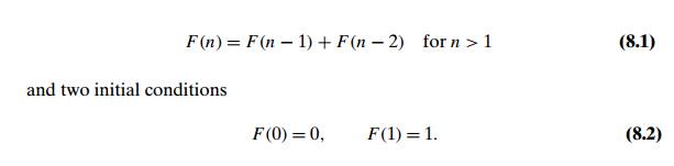
If we try to use recurrence (8.1) directly to compute the nth Fibonacci number F (n), we would have to recompute the same values of this function many times (see Figure 2.6 for an example). Note that the problem of computing F (n) is expressed in terms of its smaller and overlapping subproblems of computing F (n − 1) and F (n − 2). So we can simply fill elements of a one-dimensional array with the n + 1 consecutive values of F (n) by starting, in view of initial conditions (8.2), with 0 and 1 and using equation (8.1) as the rule for producing all the other elements. Obviously, the last element of this array will contain F (n). Single-loop pseudocode of this very simple algorithm can be found in Section 2.5.

Note that we can, in fact, avoid using an extra array to accomplish this task by recording the values of just the last two elements of the Fibonacci sequence (Problem 8 in Exercises 2.5). This phenomenon is not unusual, and we shall en-counter it in a few more examples in this chapter. Thus, although a straightforward application of dynamic programming can be interpreted as a special variety of space-for-time trade-off, a dynamic programming algorithm can sometimes be re-fined to avoid using extra space.

Certain algorithms compute the nth Fibonacci number without computing all the preceding elements of this sequence (see Section 2.5). It is typical of an algorithm based on the classic bottom-up dynamic programming approach, however, to solve all smaller subproblems of a given problem. One variation of the dynamic programming approach seeks to avoid solving unnecessary subproblems. This technique, illustrated in Section 8.2, exploits so-called memory functions and can be considered a top-down variation of dynamic programming.

Whether one uses the classical bottom-up version of dynamic programming or its top-down variation, the crucial step in designing such an algorithm remains the same: deriving a recurrence relating a solution to the problem to solutions to its smaller subproblems. The immediate availability of equation (8.1) for computing the nth Fibonacci number is one of the few exceptions to this rule.

Since a majority of dynamic programming applications deal with optimiza-tion problems, we also need to mention a general principle that underlines such applications. Richard Bellman called it the principle of optimality. In terms some-what different from its original formulation, it says that an optimal solution to any instance of an optimization problem is composed of optimal solutions to its subin-stances. The principle of optimality holds much more often than not. (To give a rather rare example, it fails for finding the longest simple path in a graph.) Al-though its applicability to a particular problem needs to be checked, of course, such a check is usually not a principal difficulty in developing a dynamic program-ming algorithm.

In the sections and exercises of this chapter are a few standard examples of dynamic programming algorithms. (The algorithms in Section 8.4 were, in fact, invented independently of the discovery of dynamic programming and only later came to be viewed as examples of this technique’s applications.) Numerous other applications range from the optimal way of breaking text into lines (e.g., [Baa00]) to image resizing [Avi07] to a variety of applications to sophisticated engineering problems (e.g., [Ber01]).