Dynamic Programming: Three Basic Examples

Three Basic Examples

The goal of this section is to introduce dynamic programming via three typical examples.

EXAMPLE 1 Coin-row problem There is a row of n coins whose values are some positive integers c₁, c₂, . . . , c_n, not necessarily distinct. The goal is to pick up the maximum amount of money subject to the constraint that no two coins adjacent in the initial row can be picked up.

Let F (n) be the maximum amount that can be picked up from the row of n coins. To derive a recurrence for F (n), we partition all the allowed coin selections into two groups: those that include the last coin and those without it. The largest amount we can get from the first group is equal to c_n + F (n − 2)—the value of the nth coin plus the maximum amount we can pick up from the first n − 2 coins. The maximum amount we can get from the second group is equal to F (n − 1) by the definition of F (n). Thus, we have the following recurrence subject to the obvious initial conditions:

We can compute F (n) by filling the one-row table left to right in the manner similar to the way it was done for the nth Fibonacci number by Algorithm Fib(n) in Section 2.5.

ALGORITHM     CoinRow(C[1..n])

//Applies formula (8.3) bottom up to find the maximum amount of money //that can be picked up from a coin row without picking two adjacent coins //Input: Array C[1..n] of positive integers indicating the coin values //Output: The maximum amount of money that can be picked up

F [0] ← 0; F [1] ← C[1] for i ← 2 to n do

F [i] ← max(C[i] + F [i − 2], F [i − 1])

return F [n]

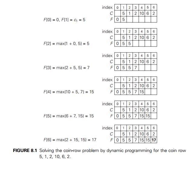
The application of the algorithm to the coin row of denominations 5, 1, 2, 10, 6, 2 is shown in Figure 8.1. It yields the maximum amount of 17. It is worth pointing

out that, in fact, we also solved the problem for the first i coins in the row given for every 1 ≤ i ≤ 6. For example, for i = 3, the maximum amount is F (3) = 7.

To find the coins with the maximum total value found, we need to back-trace the computations to see which of the two possibilities—c_n + F (n − 2) or F (n − 1)—produced the maxima in formula (8.3). In the last application of the formula, it was the sum c₆ + F (4), which means that the coin c₆ = 2 is a part of an optimal solution. Moving to computing F (4), the maximum was produced by the sum c₄ + F (2), which means that the coin c₄ = 10 is a part of an optimal solution as well. Finally, the maximum in computing F (2) was produced by F (1), implying that the coin c₂ is not the part of an optimal solution and the coin c₁ = 5 is. Thus, the optimal solution is {c₁, c₄, c₆}. To avoid repeating the same computations during the backtracing, the information about which of the two terms in (8.3) was larger can be recorded in an extra array when the values of F are computed.

Using the CoinRow to find F (n), the largest amount of money that can be picked up, as well as the coins composing an optimal set, clearly takes  $(n) time and  $ (n) space. This is by far superior to the alternatives: the straightforward top- down application of recurrence (8.3) and solving the problem by exhaustive search (Problem 3 in this section’s exercises).

EXAMPLE 2 Change-making problem Consider the general instance of the following well-known problem. Give change for amount n using the minimum number of coins of denominations d₁ < d₂ < ^{. . .} < d_m. For the coin denominations used in the United States, as for those used in most if not all other countries, there is a very simple and efficient algorithm discussed in the next chapter. Here, we consider a dynamic programming algorithm for the general case, assuming availability of unlimited quantities of coins for each of the m denominations

d₁ < d₂ < ^{. . .} < d_m where d₁ = 1.

Let F (n) be the minimum number of coins whose values add up to n; it is convenient to define F (0) = 0. The amount n can only be obtained by adding one coin of denomination d_j to the amount n − d_j for j = 1, 2, . . . , m such that n ≥ d_j . Therefore, we can consider all such denominations and select the one minimizing F (n − d_j ) + 1. Since 1 is a constant, we can, of course, find the smallest F (n − d_j ) first and then add 1 to it. Hence, we have the following recurrence for F (n):

We can compute F (n) by filling a one-row table left to right in the manner similar to the way it was done above for the coin-row problem, but computing a table entry here requires finding the minimum of up to m numbers.

ALGORITHM     ChangeMaking(D[1..m], n)

//Applies dynamic programming to find the minimum number of coins //of denominations d₁ < d₂ < ^{. . .} < d_m where d₁ = 1 that add up to a //given amount n

//Input: Positive integer n and array D[1..m] of increasing positive // integers indicating the coin denominations where D[1] = 1 //Output: The minimum number of coins that add up to n

F [0] ← 0

for i ← 1 to n do

t emp ← ∞; j ← 1

while j ≤ m and i ≥ D[j ] do

t emp ← min(F [i − D[j ]], t emp) j ← j + 1

F [i] ← t emp + 1 return F [n]

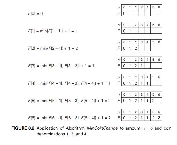
The application of the algorithm to amount n = 6 and denominations 1, 3, 4 is shown in Figure 8.2. The answer it yields is two coins. The time and space efficiencies of the algorithm are obviously O(nm) and  $(n), respectively.

To find the coins of an optimal solution, we need to backtrace the computa-tions to see which of the denominations produced the minima in formula (8.4). For the instance considered, the last application of the formula (for n = 6), the minimum was produced by d₂ = 3. The second minimum (for n = 6 − 3) was also produced for a coin of that denomination. Thus, the minimum-coin set for n = 6 is two 3’s.

EXAMPLE 3 Coin-collecting problem Several coins are placed in cells of an n × m board, no more than one coin per cell. A robot, located in the upper left cell of the board, needs to collect as many of the coins as possible and bring them to the bottom right cell. On each step, the robot can move either one cell to the right or one cell down from its current location. When the robot visits a cell with a coin, it always picks up that coin. Design an algorithm to find the maximum number of coins the robot can collect and a path it needs to follow to do this.

Let F (i, j ) be the largest number of coins the robot can collect and bring to the cell (i, j ) in the ith row and j th column of the board. It can reach this cell either from the adjacent cell (i − 1, j ) above it or from the adjacent cell (i, j − 1) to the left of it. The largest numbers of coins that can be brought to these cells are F (i − 1, j ) and F (i, j − 1), respectively. Of course, there are no adjacent cells above the cells in the first row, and there are no adjacent cells to the left of the cells in the first column. For those cells, we assume that F (i − 1, j ) and F (i, j − 1) are equal to 0 for their nonexistent neighbors. Therefore, the largest number of coins the robot can bring to cell (i, j ) is the maximum of these two numbers plus one possible coin at cell (i, j ) itself. In other words, we have the following formula for F (i, j ):

where c_ij = 1 if there is a coin in cell (i, j ), and c_ij = 0 otherwise.

Using these formulas, we can fill in the n × m table of F (i, j ) values either row by row or column by column, as is typical for dynamic programming algorithms involving two-dimensional tables.

ALGORITHM     RobotCoinCollection(C[1..n, 1..m])

//Applies dynamic programming to compute the largest number of //coins a robot can collect on an n × m board by starting at (1, 1) //and moving right and down from upper left to down right corner //Input: Matrix C[1..n, 1..m] whose elements are equal to 1 and 0 //for cells with and without a coin, respectively

//Output: Largest number of coins the robot can bring to cell (n, m) F [1, 1] ← C[1, 1]; for j ← 2 to m do F [1, j ] ← F [1, j − 1] + C[1, j ] for i ← 2 to n do

F [i, 1] ← F [i − 1, 1] + C[i, 1] for j ← 2 to m do

F [i, j ] ← max(F [i − 1, j ], F [i, j − 1]) + C[i, j ] return F [n, m]

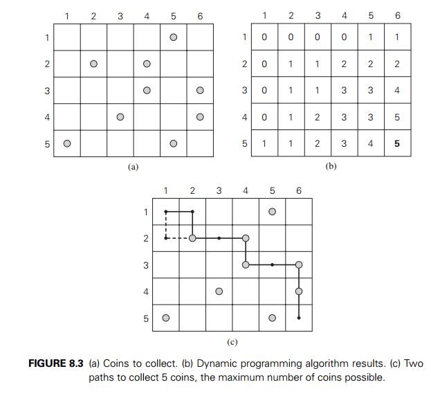
The algorithm is illustrated in Figure 8.3b for the coin setup in Figure 8.3a. Since computing the value of F (i, j ) by formula (8.5) for each cell of the table takes constant time, the time efficiency of the algorithm is  (nm). Its space efficiency is, obviously, also  (nm).

Tracing the computations backward makes it possible to get an optimal path: if F (i − 1, j ) > F (i, j − 1), an optimal path to cell (i, j ) must come down from the adjacent cell above it; if F (i − 1, j ) < F (i, j − 1), an optimal path to cell (i, j ) must come from the adjacent cell on the left; and if F (i − 1, j ) = F (i, j − 1), it can reach cell (i, j ) from either direction. This yields two optimal paths for the instance in Figure 8.3a, which are shown in Figure 8.3c. If ties are ignored, one optimal path can be obtained in  (n + m) time.

Exercises 8.1

            What does dynamic programming have in common with divide-and-conquer? What is a principal difference between them?

            Solve the instance 5, 1, 2, 10, 6 of the coin-row problem.

            a. Show that the time efficiency of solving the coin-row problem by straight-forward application of recurrence (8.3) is exponential.

            Show that the time efficiency of solving the coin-row problem by exhaustive search is at least exponential.

Apply the dynamic programming algorithm to find all the solutions to the change-making problem for the denominations 1, 3, 5 and the amount n = 9.

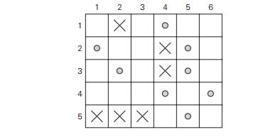
How would you modify the dynamic programming algorithm for the coin-collecting problem if some cells on the board are inaccessible for the robot? Apply your algorithm to the board below, where the inaccessible cells are shown by X’s. How many optimal paths are there for this board?

         Rod-cutting problem Design a dynamic programming algorithm for the fol-lowing problem. Find the maximum total sale price that can be obtained by cutting a rod of n units long into integer-length pieces if the sale price of a piece i units long is p_i for i = 1, 2, . . . , n. What are the time and space efficiencies of your algorithm?

         Shortest-path counting A chess rook can move horizontally or vertically to any square in the same row or in the same column of a chessboard. Find the number of shortest paths by which a rook can move from one corner of a chessboard to the diagonally opposite corner. The length of a path is measured by the number of squares it passes through, including the first and the last squares. Solve the problem

            by a dynamic programming algorithm.

            by using elementary combinatorics.

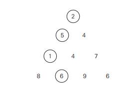
         Minimum-sum descent Some positive integers are arranged in an equilateral triangle with n numbers in its base like the one shown in the figure below for n = 4. The problem is to find the smallest sum in a descent from the triangle apex to its base through a sequence of adjacent numbers (shown in the figure by the circles). Design a dynamic programming algorithm for this problem and indicate its time efficiency.

            Binomial coefficient Design an efficient algorithm for computing the bino-mial coefficient C(n, k) that uses no multiplications. What are the time and space efficiencies of your algorithm?

            Longest path in a dag

                                                                            Design an efficient algorithm for finding the length of the longest path in a dag. (This problem is important both as a prototype of many other dynamic programming applications and in its own right because it determines the minimal time needed for completing a project comprising precedence-constrained tasks.)

                                                                            Show how to reduce the coin-row problem discussed in this section to the problem of finding a longest path in a dag.

            Maximum square submatrix Given an m × n boolean matrix B, find its largest square submatrix whose elements are all zeros. Design a dynamic programming algorithm and indicate its time efficiency. (The algorithm may be useful for, say, finding the largest free square area on a computer screen or for selecting a construction site.)

            World Series odds Consider two teams, A and B, playing a series of games until one of the teams wins n games. Assume that the probability of A winning a game is the same for each game and equal to p, and the probability of A losing a game is q = 1 − p. (Hence, there are no ties.) Let P (i, j ) be the probability of A winning the series if A needs i more games to win the series and B needs j more games to win the series.

                                                                            Set up a recurrence relation for P (i, j ) that can be used by a dynamic programming algorithm.

                                                                            Find the probability of team A winning a seven-game series if the proba-bility of it winning a game is 0.4.

                                                                            Write pseudocode of the dynamic programming algorithm for solving this problem and determine its time and space efficiencies.