Chapter: Introduction to the Design and Analysis of Algorithms : Dynamic Programming
Optimal Binary Search Trees
Optimal
Binary Search Trees
A binary search tree is one
of the most important data structures in computer science. One of its principal
applications is to implement a dictionary, a set of elements with the
operations of searching, insertion, and deletion. If probabilities
of searching for elements of
a set are knownŌĆöe.g., from accumulated data about past searchesŌĆöit is natural
to pose a question about an optimal binary search tree for which the average
number of comparisons in a search is the smallest possible. For simplicity, we
limit our discussion to minimizing the average number of comparisons in a
successful search. The method can be extended to include unsuccessful searches
as well.
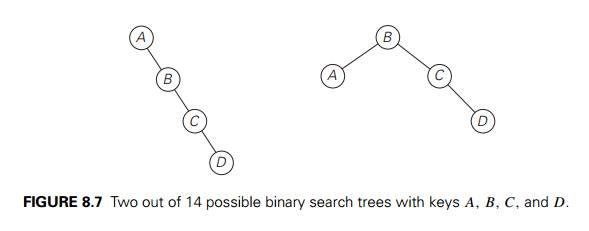
As an example, consider four
keys A, B, C, and D to be searched for with probabilities 0.1, 0.2,
0.4, and 0.3, respectively. Figure 8.7 depicts two out of 14 possible binary
search trees containing these keys. The average number of
comparisons in a successful
search in the first of these trees is 0.1 . 1 + 0.2 . 2 + 0.4 . 3 + 0.3 . 4 = 2.9, and for the second one it
is 0.1 . 2 + 0.2 . 1 + 0.4 . 2 + 0.3 . 3 = 2.1.
Neither of these two trees
is, in fact, optimal. (Can you tell which binary tree is optimal?)
For our tiny example, we
could find the optimal tree by generating all 14 binary search trees with these
keys. As a general algorithm, this exhaustive-search approach is unrealistic:
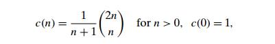
the total number of binary search trees with n keys is equal to the nth Catalan number,
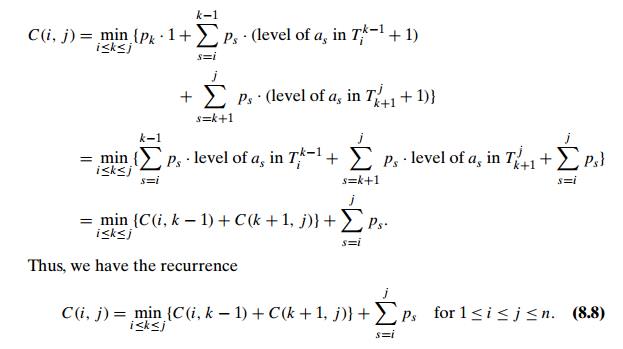
which grows to infinity as fast as 4n/n1.5 (see Problem 7 in this sectionŌĆÖs exercises). So let a1, . . . , an be distinct keys ordered from the smallest to the largest and let p1, . . . , pn be the probabilities of searching for them. Let C(i, j ) be the smallest average number of comparisons made in a successful search in a binary search tree Tij made up of keys ai, . . . , aj , where i, j are some integer indices, 1 Ōēż i Ōēż j Ōēż n. Following the classic dynamic programming approach, we will find values of C(i, j ) for all smaller instances of the problem, although we are interested just in C(1, n). To derive a recurrence underlying a dynamic programming algorithm, we will consider all possible ways to choose a root ak among the keys ai, . . . , aj . For such a binary
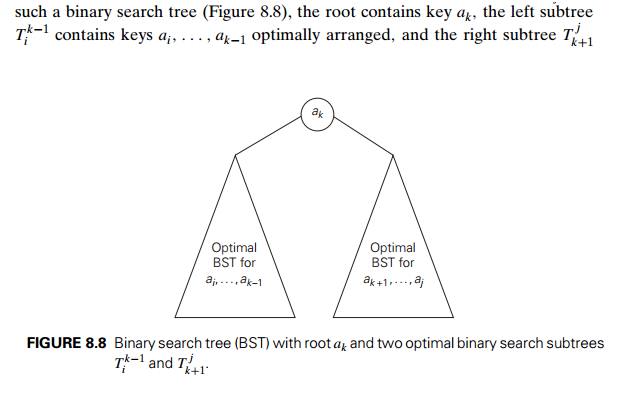
contains keys ak+1, . . . , aj also optimally arranged. (Note how we are
taking advantage of the principle of optimality here.)
If we count tree levels
starting with 1 to make the comparison numbers equal the keysŌĆÖ levels, the
following recurrence relation is obtained:
We assume in formula (8.8)
that C(i, i ŌłÆ 1) = 0 for 1 Ōēż i Ōēż n + 1, which can be interpreted as
the number of comparisons in the empty tree. Note that this formula implies
that
C(i, i) = pi for
1 Ōēż i Ōēż n,
as it should be for a
one-node binary search tree containing ai.
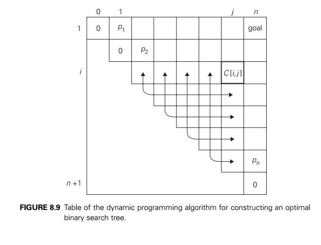
The two-dimensional table in
Figure 8.9 shows the values needed for comput-ing C(i, j ) by formula (8.8): they are in row i and the columns to the left of column j and in column j and the rows below row i. The arrows point to the pairs of en-tries
whose sums are computed in order to find the smallest one to be recorded as the
value of C(i, j ). This suggests filling the
table along its diagonals, starting with all zeros on the main diagonal and
given probabilities pi, 1 Ōēż i Ōēż n, right above it and moving
toward the upper right corner.
The algorithm we just
sketched computes C(1, n)ŌĆöthe average number of comparisons for
successful searches in the optimal binary tree. If we also want to get the
optimal tree itself, we need to maintain another two-dimensional table to
record the value of k for which the minimum in
(8.8) is achieved. The table has the same shape as the table in Figure 8.9 and
is filled in the same manner, starting with entries R(i, i) = i for 1 Ōēż i Ōēż n. When the table is filled,
its entries indicate indices of the roots of the optimal subtrees, which makes
it possible to reconstruct an optimal tree for the entire set given.
EXAMPLE
Let us
illustrate the algorithm by applying it to the four-key set we used at the beginning of this
section:
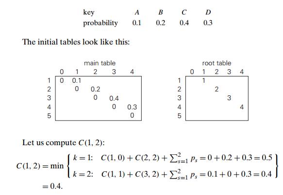
Thus, out of two possible
binary trees containing the first two keys, A and B, the root of the optimal tree has index 2
(i.e., it contains B), and the average number of
comparisons in a successful search in this tree is 0.4.
We will ask you to finish the
computations in the exercises. You should arrive at the following final tables:
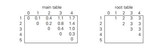
Thus, the average number of
key comparisons in the optimal tree is equal to 1.7. Since R(1, 4) = 3, the root of the optimal tree
contains the third key, i.e., C. Its left subtree is made up
of keys A and B, and its right subtree contains just key D (why?). To find the specific structure of
these subtrees, we find first their roots by consulting the root table again as
follows. Since R(1, 2) = 2, the root of the optimal tree
containing A and B is B, with A being its left child (and the root of the
one-node tree: R(1, 1) = 1). Since R(4, 4) = 4, the root of this one-node optimal tree is
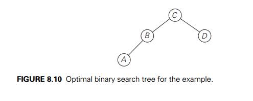
its only key D. Figure 8.10 presents the
optimal tree in its entirety.
Here is pseudocode of the
dynamic programming algorithm.
ALGORITHM OptimalBST(P [1..n])
//Finds an optimal binary
search tree by dynamic programming
//Input: An array P [1..n] of search probabilities for
a sorted list of n keys //Output: Average
number of comparisons in successful searches in the // optimal BST and table R of subtreesŌĆÖ roots in the optimal BST for i ŌåÉ 1 to n do
C[i,
i ŌłÆ 1] ŌåÉ 0 C[i, i] ŌåÉ P [i] R[i,
i] ŌåÉ i
C[n + 1,
n] ŌåÉ 0
for d ŌåÉ 1 to n ŌłÆ 1 do //diagonal count for i ŌåÉ 1 to n ŌłÆ d do
j ŌåÉ i + d minval ŌåÉ
Ōł×
for k ŌåÉ i to j do
if C[i, k ŌłÆ 1] + C[k + 1, j ] < minval
minval ŌåÉ C[i, k ŌłÆ 1] + C[k + 1, j ]; kmin ŌåÉ k R[i, j ] ŌåÉ kmin
sum ŌåÉ P [i]; for s ŌåÉ i + 1 to j do sum ŌåÉ sum + P [s] C[i, j ] ŌåÉ minval + sum
return C[1, n],
R
The algorithmŌĆÖs space
efficiency is clearly quadratic; the time efficiency of this version of the
algorithm is cubic (why?). A more careful analysis shows that entries in the
root table are always nondecreasing along each row and column. This limits
values for R(i, j ) to the range R(i, j ŌłÆ 1),
. . . , R(i + 1, j ) and makes it possible to reduce the running
time of the algorithm to (n2).
Exercises 8.3
Finish the computations started in the sectionŌĆÖs example of constructing
an optimal binary search tree.
a. Why is the time efficiency of algorithm OptimalBST cubic?
b. Why is the space efficiency of algorithm OptimalBST quadratic?
Write pseudocode for a linear-time algorithm that generates the
optimal binary search tree from the root table.
4. Devise a way to compute the
sums s=i ps, which are used in the dynamic programming
algorithm for constructing an optimal binary search tree, in constant time (per
sum).
True or false: The root of an optimal binary search tree always
contains the key with the highest search probability?
How would you construct an optimal binary search tree for a set of n keys if all the keys are equally likely to be
searched for? What will be the average number of comparisons in a successful
search in such a tree if n = 2k?
a. Show that the number of
distinct binary search trees b(n) that can be constructed for a set of n orderable keys satisfies the recurrence
relation
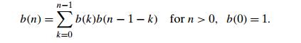
It is known that the solution to this recurrence is given by the
Catalan numbers. Verify this assertion for n = 1, 2, . . . , 5.
Find the order of growth of b(n). What implication does the answer to this
question have for the exhaustive-search algorithm for constructing an optimal
binary search tree?
Design a (n2) algorithm for finding an optimal binary search
tree.
Generalize the optimal binary search algorithm by taking into
account unsuc-cessful searches.
Write pseudocode of a memory function for the optimal binary search
tree problem. You may limit your function to finding the smallest number of key
comparisons in a successful search.
Matrix chain multiplication Consider the problem of
minimizing the total number of multiplications made in computing the product of n matrices
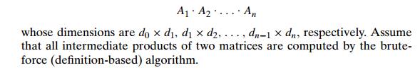
Give an example of three matrices for which the number of
multiplications in (A1 . A2) . A3 and A1 . (A2 . A3) differ at least by a factor of 1000.
How many different ways are there to compute the product of n matrices?
Design a dynamic programming algorithm for finding an optimal order
of multiplying n matrices.
Related Topics