Sorting by Counting

Sorting by Counting

As a first example of applying the input-enhancement technique, we discuss its application to the sorting problem. One rather obvious idea is to count, for each element of a list to be sorted, the total number of elements smaller than this element and record the results in a table. These numbers will indicate the positions of the elements in the sorted list: e.g., if the count is 10 for some element, it should be in the 11th position (with index 10, if we start counting with 0) in the sorted array. Thus, we will be able to sort the list by simply copying its elements to their appropriate positions in a new, sorted list. This algorithm is called comparison-counting sort (Figure 7.1).

ALGORITHM     ComparisonCountingSort(A[0..n − 1])

//Sorts an array by comparison counting

//Input: An array A[0..n − 1] of orderable elements

//Output: Array S[0..n − 1] of A’s elements sorted in nondecreasing order for i ← 0 to n − 1 do Count[i] ← 0

for i ← 0 to n − 2 do

for j ← i + 1 to n − 1 do

if A[i] < A[j ]

Count[j ] ← Count[j ] + 1 else Count[i] ← Count[i] + 1

for i ← 0 to n − 1 do S[Count[i]] ← A[i] return S

What is the time efficiency of this algorithm? It should be quadratic because the algorithm considers all the different pairs of an n-element array. More formally, the number of times its basic operation, the comparison A[i] < A[j ], is executed is equal to the sum we have encountered several times already:

Thus, the algorithm makes the same number of key comparisons as selection sort and in addition uses a linear amount of extra space. On the positive side, the algorithm makes the minimum number of key moves possible, placing each of them directly in their final position in a sorted array.

The counting idea does work productively in a situation in which elements to be sorted belong to a known small set of values. Assume, for example, that we have to sort a list whose values can be either 1 or 2. Rather than applying a general sorting algorithm, we should be able to take advantage of this additional information about values to be sorted. Indeed, we can scan the list to compute the number of 1’s and the number of 2’s in it and then, on the second pass, simply make the appropriate number of the first elements equal to 1 and the remaining elements equal to 2. More generally, if element values are integers between some lower bound l and upper bound u, we can compute the frequency of each of those values and store them in array F [0..u − l]. Then the first F [0] positions in the sorted list must be filled with l, the next F [1] positions with l + 1, and so on. All this can be done, of course, only if we can overwrite the given elements.

Let us consider a more realistic situation of sorting a list of items with some other information associated with their keys so that we cannot overwrite the list’s elements. Then we can copy elements into a new array S[0..n − 1] to hold the sorted list as follows. The elements of A whose values are equal to the lowest possible value l are copied into the first F [0] elements of S, i.e., positions 0 through F [0] − 1; the elements of value l + 1 are copied to positions from F [0] to (F [0] + F [1]) − 1; and so on. Since such accumulated sums of frequencies are called a distribution in statistics, the method itself is known as distribution counting.

EXAMPLE Consider sorting the array

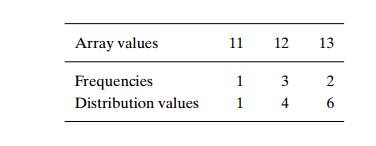
whose values are known to come from the set {11, 12, 13} and should not be overwritten in the process of sorting. The frequency and distribution arrays are as follows:

Note that the distribution values indicate the proper positions for the last occur-rences of their elements in the final sorted array. If we index array positions from 0 to n − 1, the distribution values must be reduced by 1 to get corresponding element positions.

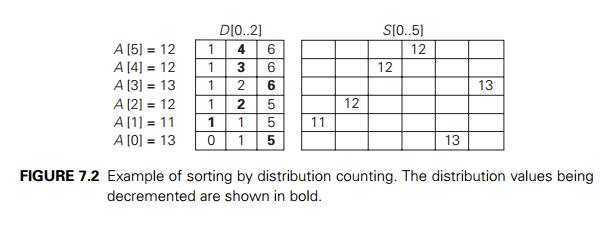
It is more convenient to process the input array right to left. For the example, the last element is 12, and, since its distribution value is 4, we place this 12 in position 4 − 1 = 3 of the array S that will hold the sorted list. Then we decrease the 12’s distribution value by 1 and proceed to the next (from the right) element in the given array. The entire processing of this example is depicted in Figure 7.2.

Here is pseudocode of this algorithm.

ALGORITHM     DistributionCountingSort(A[0..n − 1], l, u)

//Sorts an array of integers from a limited range by distribution counting //Input: An array A[0..n − 1] of integers between l and u (l ≤ u) //Output: Array S[0..n − 1] of A’s elements sorted in nondecreasing order for j ← 0 to u − l do D[j ] ← 0 //initialize frequencies for i ← 0 to n − 1 do D[A[i] − l] ← D[A[i] − l] + 1 //compute frequencies

for j ← 1 to u − l do D[j ] ← D[j − 1] + D[j ]      //reuse for distribution

for i ← n − 1 downto 0 do

j ← A[i] − l

S[D[j ] − 1] ← A[i]

D[j ] ← D[j ] − 1

return S

Assuming that the range of array values is fixed, this is obviously a linear algorithm because it makes just two consecutive passes through its input array A. This is a better time-efficiency class than that of the most efficient sorting algorithms—mergesort, quicksort, and heapsort—we have encountered. It is im-portant to remember, however, that this efficiency is obtained by exploiting the specific nature of inputs for which sorting by distribution counting works, in addi-tion to trading space for time.

Exercises 7.1

            Is it possible to exchange numeric values of two variables, say, u and v, without using any extra storage?

            Will the comparison-counting algorithm work correctly for arrays with equal values?

Assuming that the set of possible list values is {a, b, c, d}, sort the following list in alphabetical order by the distribution-counting algorithm:

            Is the distribution-counting algorithm stable?

            Design a one-line algorithm for sorting any array of size n whose values are n distinct integers from 1 to n.

            The ancestry problem asks to determine whether a vertex u is an ancestor of vertex v in a given binary (or, more generally, rooted ordered) tree of n vertices. Design a O(n) input-enhancement algorithm that provides sufficient information to solve this problem for any pair of the tree’s vertices in constant time.

            The following technique, known as virtual initialization, provides a time-efficient way to initialize just some elements of a given array A[0..n − 1] so that for each of its elements, we can say in constant time whether it has been initialized and, if it has been, with which value. This is done by utilizing a variable count er for the number of initialized elements in A and two auxiliary arrays of the same size, say B[0..n − 1] and C[0..n − 1], defined as follows. B[0], . . . , B[count er − 1] contain the indices of the elements of A that were initialized: B[0] contains the index of the element initialized first, B[1] contains the index of the element initialized second, etc. Furthermore, if A[i] was the kth element (0 ≤ k ≤ count er − 1) to be initialized, C[i] contains k.

            Sketch the state of arrays A[0..7], B[0..7], and C[0..7] after the three as-signments

                                                                            In general, how can we check with this scheme whether A[i] has been initialized and, if it has been, with which value?

            Least distance sorting There are 10 Egyptian stone statues standing in a row in an art gallery hall. A new curator wants to move them so that the statues are ordered by their height. How should this be done to minimize the total distance that the statues are moved? You may assume for simplicity that all the statues have different heights. [Azi10]

            a. Write a program for multiplying two sparse matrices, a p × q matrix A and a q × r matrix B.

b. Write a program for multiplying two sparse polynomials p(x) and q(x) of degrees m and n, respectively.