The Transportation Algorithm

THE TRANSPORTATION ALGORITHM

The transportation algorithm follows the exact steps of the simplex method (Chapter 3). However, instead of using the regular simplex tableau, we take advantage of the special structure of the transportation model to organize the computations in a more convenient form.

The special transportation algorithm was developed early on when hand computations were the norm and the shortcuts were warranted. Today, we have powerful computer codes that can solve a transportation model of any size as a regular Lp' Nevertheless, the transportation algorithm, aside from its historical significance, does pro-vide insight into the use of the theoretical primal-dual relationships (introduced in Section 4.2) to achieve a practical end result, that of improving hand computations. The 5. exercise is theoretically intriguing.

The details of the algorithm are explained using the following numeric example.

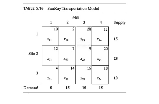
Example 5.3-1         (SunRay Transport)

SunRay Transport Company ships truckloads of grain from three silos to four mills. The supply (in truckloads) and the demand (also in truckloads) together with the unit transportation costs per truckload on the different routes are summarized in the transportation model in Table 5.16. The unit transportation costs, eij, (shown in the northeast corner of each box) are in hundreds of dollars. The model seeks the minimum-cost shipping schedule Xij between silo i and mill j (i = 1,2,3; j = 1,2,3,4).

Summary of the Transportation Algorithm. The steps of the transportation algorithm are exact parallels of the simplex algorithm.

Step 1. Determine a starting basic feasible solution, and go to step 2.

Step 2. Use the optimality condition of the simplex method to determine the entering variable from among all the nonbasic variables. If the optimality condition is satisfied, stop. Otherwise, go to step 3.

Step 3. Use the feasibility condition of the simplex method to determine the leaving variable from among all the current basic variables, and find the new basic solution. Return to step 2.

1. Determination of the Starting Solution

A general transportation model with m sources and n destinations has m + n constraint equations, one for each source and each destination. However, because the transportation model is always balanced (sum of the supply = sum of the demand), one of these equations is redundant. Thus, the model has m + n - 1 independent constraint equations, which means that the starting basic solution consists of m + n - 1 basic variables. Thus, in Example 5.3-1, the starting solution has 3 + 4 - 1 = 6 basic variables.

The special structure of the transportation problem allows securing a nonartificiaI starting basic solution using one of three methods:

a)     Northwest-corner method

b)    Least-cost method

c)     Vogel approximation method

. The three methods differ in the "quality" of the starting basic solution they produce, in the sense that a better starting solution yields a smaller objective value. In general, though not always, the Vogel method yields the best starting basic solution, and the northwest-corner method yields the worst. The tradeoff is that the northwest-corner method involves the least amount of computations.

Northwest-Corner Method. The method starts at the northwest-corner cell (route) of the tableau (variable x₁₁).

Step 1. Allocate as much as possible to the selected cell, and adjust the associated amounts of supply and demand by subtracting the allocated amount.

Step 2. Cross out the row or column with zero supply or demand to indicate that no further assignments can be made in that row or column. If both a row and a column net to zero simultaneously, cross out one only, and leave a zero sup-ply (demand) in the uncrossed-out TOW (column).

Step 3. If exactly one row or column is left uncrossed out, stop. Otherwise, move to the cell to the right if a column has just been crossed out or below if a row has been crossed out. Go to step 1.

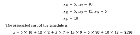
Example 5.3-2

The application of the procedure to the model of Example 5.3-1 gives the starting basic solution in Table 5.17. The arrows show the order in which the allocated amounts are generated.

The starting basic solution is

Least-Cost Method. The least-cost method finds a better starting solution by concentrating on the cheapest routes. The method assigns as much as possible to the cell with the smallest unit cost (ties are broken arbitrarily). Next, the satisfied row or column is crossed out and the amounts of supply and demand are adjusted accordingly.

If both a row and a column are satisfied simultaneously, only one is crossed out, the same as in the northwest-corner method. Next, look for the uncrossed-out cell with the smallest unit cost and repeat the process until exactly one row or column is left uncrossed out.

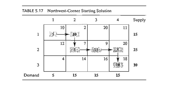
Example 5.3-3

The least-cost method is applied to Example 5.3-1 in the following manner:

1. Cell (1, 2) has the least unit cost in the tableau (= $2). The most that can be shipped through (1,2) is X₁₂ = 15 truckloads, which happens to satisfy both row 1 and column 2 simultaneously. We arbitrarily cross out column 2 and adjust the supply in row 1 to 0.

2. Cell (3,1) has the smallest uncrossed-out unit cost (= $4). Assign X₃₁ = 5, and cross out column 1 because it is satisfied, and adjust the demand of row 3 to 10 - 5 = 5 truckloads.

3. Continuing in the same manner, we successively assign 15 truckloads to cell (2, 3), 0 truckloads to cell (1,4), 5 truckloads to cell (3, 4), and 10 truckloads to cell (2,4) (verify!).

The resulting starting solution is summarized in Table 5.18. The arrows show the order in which the allocations are made. The starting solution (consisting of 6 basic variables) is x₁₂ = 15, x₁₄ = 0, x₂₃ = 15, x₂₄ = 10, x₃₁ = 5, x₃₄ = 5. The associated objective value is

z =  15 X 2 + 0 x 11 + 15 x 9 + 10 x 20 + 5 x 4 + 5 x 18 = $475

The quality of the least-cost starting solution is better than that of the northwest-corner method (Example 5.3-2) because it yields a smaller value of z ($475 versus $520 in the northwest-corner method).

Vogel Approximation Method (VAM). VAM is an improved version of the least-cost method that generally, but not always, produces better starting solutions.

Step 1. For each row (column), determine a penalty measure by subtracting the smallest unit cost element in the row (column) from the next smallest unit cost element in the same row (column).

Step 2. Identify the row or column with the largest penalty. Break ties arbitrarily. Allocate as much as possible to the variable with the least unit cost in the selected row or column. Adjust the supply and demand, and cross out the satisfied row or column. If a row and a column are satisfied simultaneously, only one of the two is crossed out, and the remaining row (column) is assigned zero supply (demand).

Step 3.

(a) If exactly one row or column with zero supply or demand remains un-crossed out, stop.

(b) If one row (column) with positive supply (demand) remains uncrossed out, determine the basic variables in the row (column) by the least-cost method. Stop.

(c) If all the uncrossed out rows and columns have (remaining) zero supply and demand, determine the zero basic variables by the least-cost method. Stop.

(d) Otherwise, go to step 1.

Example 5.3-4

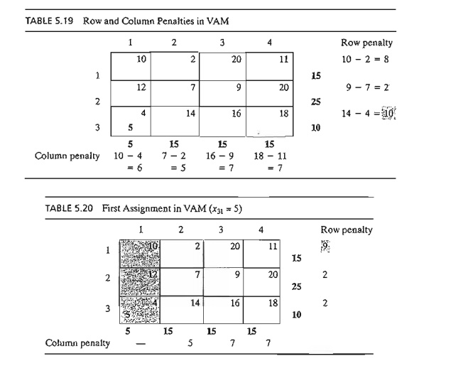
VAM is applied to Example 5.3-1. Table 5.19 computes the first set of penalties.

Because row 3 has the largest penalty (= 10) and cell (3, 1) has the smallest unit cost in that row, the amount 5 is assigned to x₃₁. Column 1 is now satisfied and must be crossed out. Next, new penalties are recomputed as in Table 5.20.

Table 5.20 shows that row 1 has the highest penalty (= 9). Hence, we assign the maximum amount possible to cell (1,2), which yields x₁₂ = 15 and simultaneously satisfies both row 1 and 5. column 2. We arbitrarily cross out column 2 and adjust the supply in row 1 to zero.

Continuing in the same manner, row 2 will produce the highest penalty (= 11), and we as-sign x₂₃ = 15, which crosses out column 3 and leaves 10 units in row 2. Only column 4 is left, and it has a positive supply of 15 units. Applying the least-cost method to that column, we successively assign x₁₄ = 0, x₃₄ = 5, and x₂₄ = 10 (verify!). The associated objective value for this solution is

z =  15 x 2 + 0 x 11 + 15 x 9 + 10 x 20 + 5 x 4 + 5 x 18 = $475

This solution happens to have the same objective value as in the least-cost method.

2. Iterative Computations of the Transportation Algorithm

After determining the starting solution (using any of the three methods in Section 5.3.1), we use the following algorithm to determ~ne the optimum solution:

Step 1. Use the simplex optimality condition to determine the entering variable as the current nonbasic variable that can improve the solution. If the optimality condition is satisfied, stop. Otherwise, go to step 2.

Step 2. Determine the leaving variable using the simplex feasibility condition. Change the basis, and return to step 1.

The optimality and feasibility conditions do not involve the familiar row operations used in the simplex method. Instead, the special structure of the transportation model allows simpler computations.

Example 5.3-5

Solve the transportation model of Example 5.3-1, starting with the northwest-corner solution.

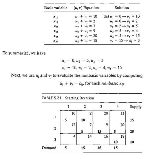
Table 5.21 gives the northwest-corner starting solution as determined in Table 5.17, Example 5.3-2.

The determination of the entering variable from among the current nonbasic variables (those that are not part of the starting basic solution) is done by computing the nonbasic coeffi-cients in the z-row, using the method of multipliers (which, as we show in Section 5.3.4, is rooted in LP duality theory).

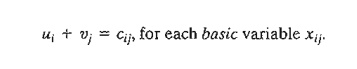
In the method of multipliers, we associate the multipliers Ui and v; with row i and column j of the transportation tableau. For each current basic variable Xi;, these multipliers are shown in Section 5.3.4 to satisfy the following equations:

u_i  + v_j = c_ij, for each basic x_ij

As Table 5.21 shows, the starting solution has 6 basic variables, which leads to 6 equations in 7 unknowns. To solve these equations, the method of multipliers calls for arbitrarily setting any u_i = 0, and then solving for the remaining variables as shown below.

The results of these evaluations are shown in the following table:

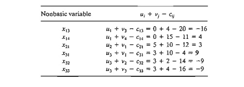
The preceding information, together with the fact that u_i + v_j - c_ij = 0 for each basic x_ij, is actually equivalent to computing the z-row of the simplex tableau, as the following summary shows.

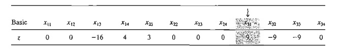
Because the transportation model seeks to minimize cost, the entering variable is the one having the most positive coefficient in the z-row. Thus, x₃₁ is the entering variable.

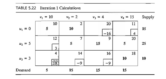
The preceding computations are usually done directly on the transportation tableau as shown in Table 5.22, meaning that it is not necessary really to write the (u, v)-equations explicitly. Instead, we start by setting u₁ = 0. Then we can compute the v-values of all the columns that have basic variables in row I-namely, v_I and v₂. Next, we compute u₂ based on the (u, v)-equation of basic x₂₂. Now, given u₂, we can compute v₃ and v_4. Finally, we determine u₃ using the basic equation of x₃₃. Once all the u's and v's have been determined, we can evaluate the nonbasic variables by computing u_i + v_j - c_ij for each nonbasic X_ij. These evaluations are shown in Table 5.22 in the boxed southeast corner of each cell.

Having identified x₃₁ as the entering variable, we need to detennine the leaving variable. Remember that if x₃₁ enters the solution to become basic, one of the current basic variables must leave as nonbasic (at zero level).

The selection of x₃₁ as the entering variable means that we want to ship through this route because it reduces the total shipping cost. What is the most that we can ship through the new route? Observe in Table 5.22 that if route (3, 1) ships () units (i.e., x₃₁ = Ф), then the maximum value of Ф is determined based on two conditions.

a)     Supply limits and demand requirements remain satisfied.

b)    Shipments through all routes remain nonnegative.

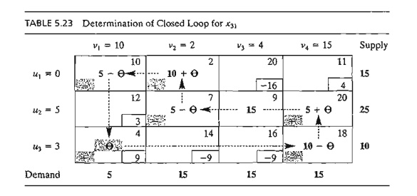
These two conditions determine the maximum value of Ф and the leaving variable in the following manner. First, construct a closed loop that starts and ends at the entering variable cell, (3, 1). The loop consists of connected horizontal and vertical segments only (no diagonals are al-lowed).7 Except for the entering variable cell, each corner of the closed loop must coincide with a basic variable. Table 5.23 shows the loop for x₃₁. Exactly one loop exists for a given entering variable.

Next, we assign the amount Ф  to the entering variable cell (3, 1). For the supply and demand limits to remain satisfied, we must alternate between subtracting and adding the amount Ф at the successive corners of the loop as shown in Table 5.23 (it is immaterial whether the loop is traced in a clockwise or counterclockwise direction). For Ф ≥ 0, the new values of the variables then remain nonnegative if

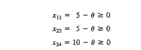
The corresponding maximum value of Ф is 5, which occurs when both x₁₁ and x₂₂ reach zero level. Because only one current basic variable must leave the basic solution, we can choose either x₁₁ or x₂₂ as the leaving variable. We arbitrarily choose X₁₁ to leave the solution.

The selection of x₃₁ (= 5) as the entering variable and x₁₁ as the leaving variable requires adjusting the values of the basic variables at the corners of the closed loop as Table 5.24 shows. Because each unit shipped through route (3, 1) reduces the shipping cost by $9 (= u₃ + v₁ - c₃₁), the total cost associated with the new schedule is $9 X 5 = $45 less than in the previous schedule. Thus, the new cost is $520 - $45 = $475.

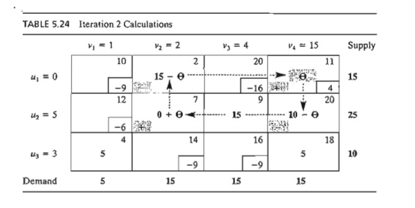
Given the new basic solution, we repeat the computation of the multipliers u and v, as Table 5.24 shows. The entering variable is x₁₄. The closed loop shows that x₁₄ = 10 and that the leaving variable is x₂₄.

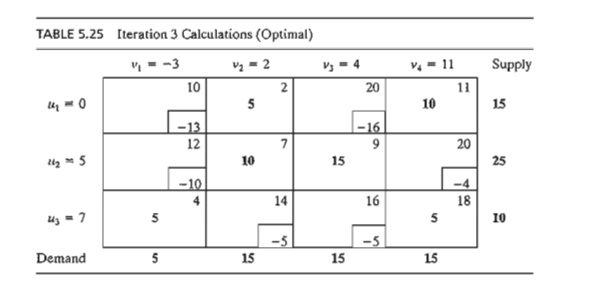
The new solution, shown in Table 5.25, costs $4 X 10 = $40 less than the preceding one, thus yielding the new cost $475 - $40 = $435. The new u_i + v_j - c_ij are now negative for all nonbasic x_ij. Thus, the solution in Table 5.25 is optimal.

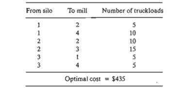
The following table summarizes the optimum solution.

TORA Moment.

From Solve/Modiy Menu , select Solve -> Iterations and choose one of the three methods (northwest corner, least cost or Vogel) to start the transportation model iterations. The iterations module offers two useful interactive features:

1. You can set any u or v to zero before generating Iteration 2 (the default is u₁ = 0). Observe then that although the values of u_i and v_j change, the evaluation of the nonbasic cells (= u_j + v_j - c_ij) remains the same. This means that, initially, any u or v can be set to zero (in fact, any value) without affecting the optimality calculations.

2. You can test your understanding of the selection of the closed loop by clicking (in any order) the corner cells that comprise the path. If your selection is correct, the cell will change color (green for entering variable, red for leaving variable, and gray otherwise).

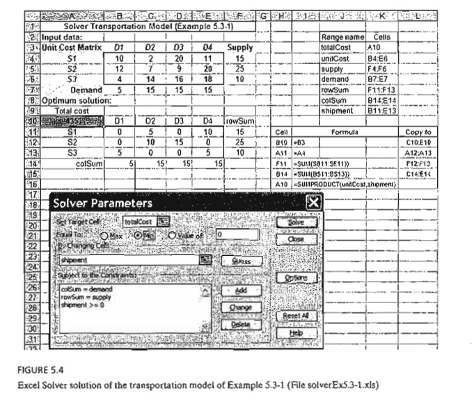
Solver Moment.

Entering the transportation model into Excel spreadsheet is straightforward. Figure 5.4 provides the Excel Solver template for Example 5.3-1 (file solverEx5.3-l.xls), together with all the formulas and the definition of range names.

In the input section, data include unit cost matrix (cells B4:E6), source names (cells A4:A6), destination names (cells B3:E3), supply (cells F4:F6), and demand (cells B7:E7). In the output section, cells B11:E13 provide the optimal solution in matrix form. The total cost formula is given in target cell A10.

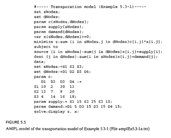
AMPl Moment.

Figure 5.5 provides the AMPL model for the transportation model of Example 5.3-1 (file amplEx5.3-1a.txt). The names used in the model are self-explanatory. Both the constraints and the objective function follow the format of the LP model presented in Example 5.1-I.

The model uses the sets sNodes and dNodes to conveniently allow the use of the alphanumeric set members {s1, s2, s3} and {Dl, D2, D3, D4} which are entered in the data section. All the input data are then entered in terms of these set members as shown in Figure 5.5.

Although the alphanumeric code for set members is more readable, generating them for large problems may not be convenient. File ampIExS.3-1b shows how the same sets can be defined as {1 .. m) and {1 .. n}, where m and n represent the number of sources and the number of destinations. By simply assigning numeric values for In and n, the sets are automatically defined for any size model.

The data of the transportation model can be retrieved from a spreadsheet (file TM.xls) using the AMPL table statement. File amplEx3S1c.txt provides the details. To study this model, you will need to review the material in Section A.5.5.

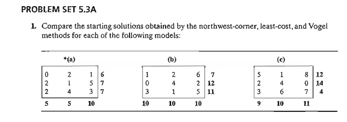
PROBLEM SET 5.3B

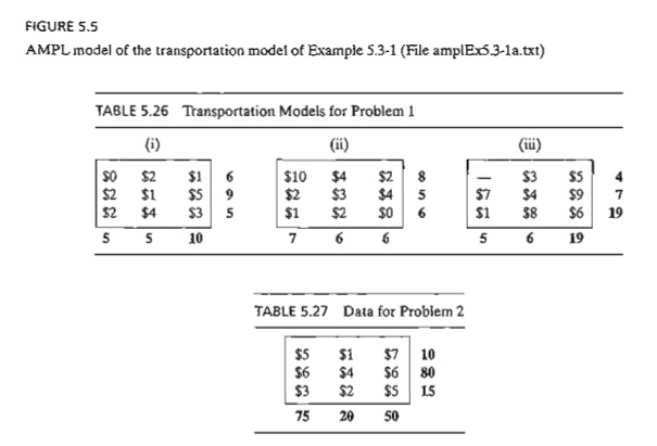
1. Consider the transportation models in Table 5.26.

a)     Use the northwest-corner method to find the starting solution.

b)    Develop the iterations that lead to the optimum solution.

c)     TO RA Experiment. Use TORA's Iterations module to compare the effect of using the northwest-corner rule, least-cost method, and Vogel method on the number of iterations leading to the optimum solution.

d)    Solver Experiment. Solve the problem by modifying file solverEx5.3-l.xls.

2. AMPL Experiment. Solve the problem by modifying file ampIEx5.3-lb.txt.

In the transportation problem in Table 5.27, the total demand exceeds the total supply.

Suppose that the penalty costs per unit of unsatisfied demand are $5, $3, and $2 for destinations 1,2, and 3, respectively. Use the least-cost starting solution and compute the iterations leading to the optimum solution.

3. In Problem 2, suppose that there are no penalty costs, but that the demand at destination 3 must be satisfied completely.

a)     Find the optimal solution.

b)    Solver Experiment. Solve the problem by modifying file solverExS.3-l.xls.

c)     AMPL Experiment. Solve the problem by modifying file ampIEx5.3b-l.txt.

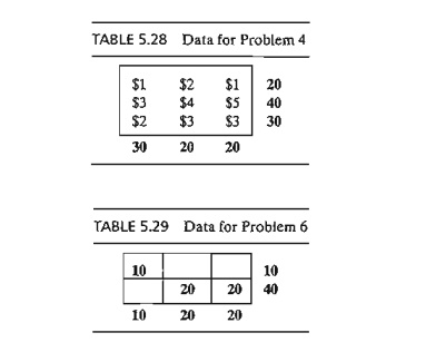
4. In the unbalanced transportation problem in Table 5.28, if a unit from a source is not shipped out (to any of the destinations), a storage cost is incurred at the rate of $5, $4, and $3 per unit for sources 1,2, and 3, respectively. Additionally, all the supply at source 2 must be shipped out completely to make room for a new product. Use Vogel's starting solution and determine all the iterations leading to the optimum ship-ping schedule.

*5. In a 3 X 3 transportation problem, let x_ij be the amount shipped from source i to destination j and let c_ij be the corresponding transportation cost per unit. The amounts of supply at sources 1,2, and 3 are 15,30, and 85 units, respectively, and the demands at destinations 1,2, and 3 are 20,30, and 80 units, respectively. Assume that the starting northwest-corner solution is optimal and that the associated values of the multipliers are given as u₁ = -2, u₂ = 3, u₃ = 5, v₁ = 2, v₂ = 5, and v₃ = 10.

(a) Find the associated optimal cost.

(b) Determine the smallest value of Gij for each nonbasic variable that will maintain the optimality of the northwest-corner solution.

6. The transportation problem in Table 5.29 gives the indicated degenerate basic solution (i.e., at least one of the basic variables is zero). Suppose that the multipliers associated with this solution are u₁ = 1, u₂ = -1, v₁ = 2, v₂ = 2, and v₃ = 5 and that the unit cost for all (basic and nonbasic) zero x_ij variables is given by

(a)     If the given solution is optimal, determine the associated optimal value of the objective function.

(b)     Determine the value of () that will guarantee the optimality of the given solution.

on      (Hint: Locate the zero basic variable.)

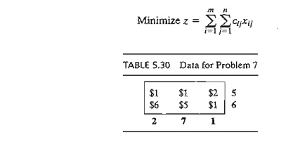
7.       Consider the problem

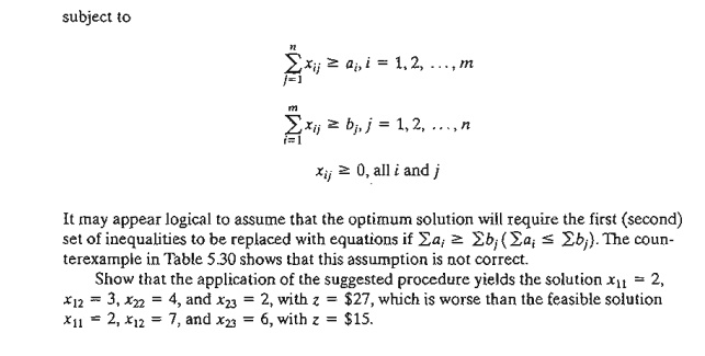
3. Simplex Method Explanation of the Method of Multipliers

The relationship between the method of multipliers and the simplex method can be explained based on the primal-dual relationships (Section 4.2). From the special structure of the LP representing the transportation model (see Example 5.1-1 for an illustra-tion), the associated dual problem can be written as

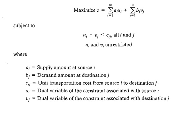
From Formula 2, Section 4.2.4, the objective-function coefficients (reduced costs) of the variable x_ij equal the difference between the left- and right-hand sides of the corresponding dual constraint-that is, u_i + v_j - c_ij. However, we know that this quantity must equal zero for each basic variable, which then produces the following result:

There are m + n - 1 such equations whose solution (after assuming an arbitrary value u₁ = 0) yields the multipliers u_i and v_j. Once these multipliers are computed, the entering variable is determined from all the nonbasic variables as the one having the largest positive u_i + v_j - c_ij.

The assignment of an arbitrary value to one of the dual variables (i.e., u₁ = 0) may appear inconsistent with the way the dual variables are computed using Method 2 in Section 4.2.3. Namely, for a given basic solution (and, hence, inverse), the dual values must be unique. Problem 2, Set 5.3c, addresses this point.

PROBLEM SET 5.3C

1. Write the dual problem for the LP of the transportation problem in Example 5.3-5 (Table 5.21). Compute the associated optimum dual objective value using the optimal dual values given in Table 5.25, and show that it equals the optimal cost given in the example.

2. In the transportation model, one of the dual variables assumes an arbitrary value. This means that for the same basic solution, the values of the associated dual variables are not unique. The result appears to contradict the theory of linear programming, where the dual values are determined as the product of the vector of the objective coefficients for the basic variables and the associated inverse basic matrix (see Method 2, Section 4.2.3). Show that for the transportation model, although the inverse basis is unique, the vector of basic objective coefficients need not be so. Specifically, show that if C_ij is changed to c_ij + k for all i and j, where k is a constant, then the optimal values of x_ij will remain the same. Hence, the use of an arbitrary value for a dual variable is implicitly equivalent to assuming that a specific constant k is added to all c_ij.